Click SigmaXL > Templates & Calculators > Control
Chart Templates > Average Run Length (ARL)
Calculators >CUSUM ARL. This template is also
located at SigmaXL > Control Charts > Control
Chart Templates> Average Run Length (ARL)
Calculators >CUSUM ARL.
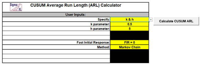
The default template settings are Specify =
k
& h, k parameter = 0.5, h parameter = 5,
Fast Initial Response: FIR = 0, Method =
Markov Chain.
Notes: Parameters to be specified will
be shown in yellow highlight, otherwise they are
hidden. The CUSUM parameter k is the reference (or
slack) value, typically set to 0.5. It sets the size
of mean shift (2k sigma) that you would like to
detect quickly, so 0.5 denotes rapid detection of a
shift in mean = 1 sigma. Alternatively, Woodall
&Faltin [4] recommend larger k values (e.g., k =
0.9) to avoid false alarms and detect shifts of
practical significance.
The CUSUM parameter h is the decision
interval, typically set to 4 or 5.
FIR sets the initial CUSUM statistic so
that it improves the sensitivity to a mean shift at
startup. Note that if the process is in control when
the CUSUM is started but shifts out of control
later, the more appropriate ARL for such a case
would be FIR=0. See Montgomery [3], pages 426-427.
Markov Chain approximation is fast and
accurate to compute ARLs. Monte Carlo simulation
allows you to assess robustness to nonnormality and
also produces the table of Run Length Standard
Deviation and Percentiles (scroll right to view).
For further details on the Markov Chain
approximation see Hawkins [1] and Lucas [2]. Monte
Carlo simulation uses the Pearson Family of
distributions to match the specified skewness and
kurtosis.
The CUSUM ARL is for a two-sided chart
with zero-state, i.e., the shift is assumed to occur
at the start. The mean and standard deviation are
also assumed to be known. This will not likely be
the case in use, but is still useful for determining
parameter settings and comparison of ARL across
chart types.
All ARL calculations for CUSUM use a
standardized in-control mean=0 and sigma=1.
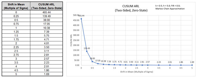
Click the Calculate CUSUM ARL button to
reproduce the ARL table and chart.
The ARL0 (in-control ARL with 0 shift in mean)
for the CUSUM chart with these settings is 465.44.
The ARL1 for a small 1 sigma shift in mean is 10.38.
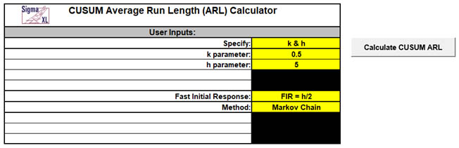
Now we will evaluate CUSUM with the same parameters,
but use the Fast Initial Response option. Select
Specify = k & h. Enter k parameter = 0.5,
h parameter = 5, Fast Initial ResponseFIR = h/2, Method = Markov Chain.
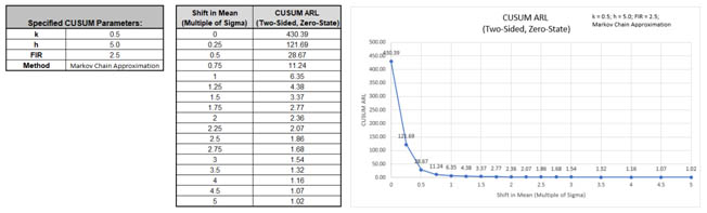
Click the Calculate CUSUM ARL button to
produce the ARL table and chart for these settings.
The ARL0 for the CUSUM chart with these
settings is 430.39 which is slightly lower than the
FIR = 0 setting, so slightly higher false alarm
rate. The ARL1 for a small 1 sigma shift in mean is
6.35 which is faster than the 10.38 for FIR = 0.
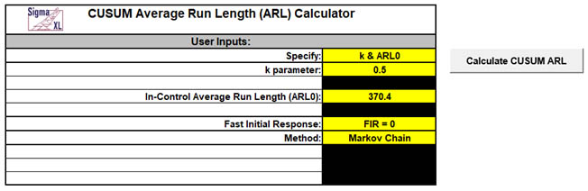
Now we will specify the CUSUM k parameter = 0.5 with
a Shewhart ARL0 value of 370.4 and solve for the h
parameter. Enter Specify = k & ARL0, k
parameter = 0.5, In-Control Average Run
Length (ARL0) = 370.4, Fast Initial Response
FIR = 0, Method = Markov Chain.
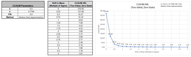
Click the Calculate CUSUM ARL button to
produce the CUSUM Parameters, ARL table and chart
for these settings.
The ARL0 for the CUSUM chart with these
settings is 370.4 as specified. The h parameter
solved to obtain this ARL0 value is 4.7749. The ARL1
for a small 1 sigma shift in mean is 9.93 so is much
faster to detect than the ARL1 of 43.89 for
Shewhart Individuals and close to the Monte
Carlo ARL1 of 9.7 for
Shewhart Individuals with 8 tests for special
causes.
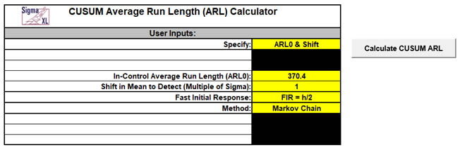
Next, we will specify a Shewhart ARL0 value of
370.4, with a desired optimization to detect a 1
sigma shift in mean and use Fast Initial Response.
The calculator will solve for the optimal k and h
parameters. Enter Specify = ARL0 & Shift,
In-Control Average Run Length (ARL0) = 370.4,
Shift in Mean to Detect (Multiple of Sigma) = 1,
Fast Initial ResponseFIR = h/2, Method =
Markov Chain.
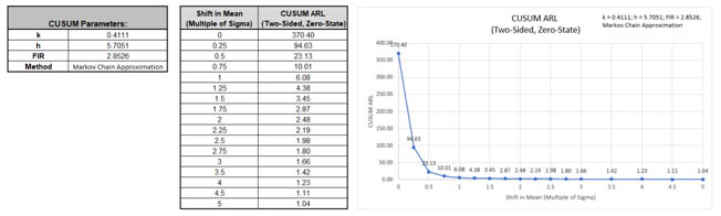
Note: Since both k and h are solved,
this takes about 20-30 seconds to compute.
Click the Calculate CUSUM ARL button to
produce the CUSUM Parameters, ARL table and chart
for these settings.
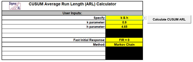
As an alternative to using the CUSUM to rapidly
detect small shifts in mean, Woodall & Faltin [4]
recommend larger k values to avoid false alarms and
detect shifts of practical significance. Enter
Specify = k & h, k parameter = 0.9, h
parameter = 4.65, Fast Initial ResponseFIR = 0, Method = Markov Chain.
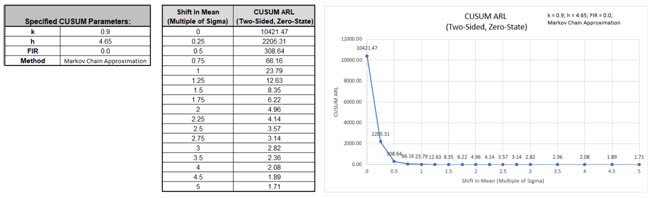
Click the Calculate CUSUM ARL button to
produce the CUSUM Parameters, ARL table and chart
for these settings.
This gives large ARL values for shift in mean
<= 1 sigma and small ARLvalues for a shift in mean
>= 1.5 sigma.
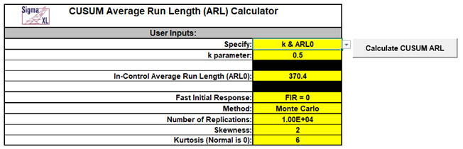
Now we will use Monte Carlo simulation to obtain
approximate Run Length standard deviation and
percentiles using the CUSUM k parameter = 0.5 with a
Shewhart ARL0 value of 370.4. Enter Specify =
k & ARL0, k parameter = 0.5, In-Control
Average Run Length (ARL0) = 370.4, Fast
Initial Response FIR = 0, Method =
Monte
Carlo, Number of Replications = 1e4,
Skewness = 0, Kurtosis (Normal is 0) = 0.
Note: The CUSUM h parameter will be
solved first using the Markov Chain approximation
and assumes a Normal distribution, so will match the
4.7749 value previously calculated above (6).
Click the Calculate CUSUM ARL button to
produce the CUSUM Parameters, Monte Carlo
approximate ARL table, ARL chart and Run Length
Standard Deviation and Percentiles table. Monte
Carlo simulation with 10,000 (1e4) replications will
take about a minute to run.
The additional run length statistics show the
large variation of run length values. The MRL0 = 255
(in-control median run length with 0 shift in
process mean).
Note: The results will vary slightly
since this is Monte Carlo simulation.
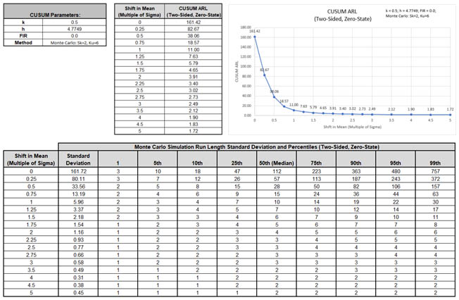
We will now assess robustness to nonnormality using
Monte Carlo simulation and compare to Shewhart and
EWMA charts. Enter Specify = k & ARL0, k
parameter = 0.5, In-Control Average Run
Length (ARL0) = 370.4, Fast Initial ResponseFIR = 0, Method = Monte Carlo, Number of
Replications = 1e4, Skewness = 2,
Kurtosis (Normal is 0) = 6.
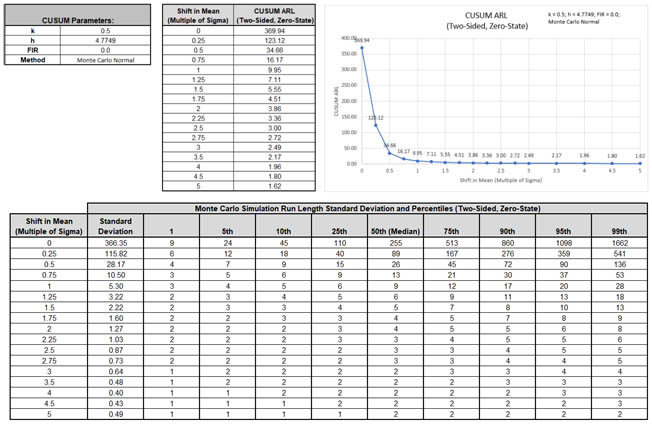
Click the Calculate CUSUM ARL button to
produce the CUSUM Parameters, Monte Carlo
approximate ARL table, ARL chart and Run Length
Standard Deviation and Percentiles table:
ARL0 is approximately 161.4 which is a 2.3 x
increase (370.4/161.4) in false alarms compared to
Normal but is a much better performance than the
ARL0 = 54.6 result for
Shewhart Individuals.
Stoumbos and Reynolds [5] recommend
setting h=6.148 (with k=0.5) as a way to improve the
CUSUM robustness to non-normality.
Template Notes:
Specify CUSUM parameters: k & h, k &ARL0 or
ARL0& Shift using the drop-down list. Parameters to
be specified will be shown in yellow highlight,
otherwise they are hidden.
If applicable, enter the CUSUM parameter k. This is
the reference (or slack) value, typically set to 0.5. It
sets the size of mean shift (2k sigma) that you would
like to detect quickly, so 0.5 denotes rapid detection
of a shift in mean = 1 sigma. Alternatively, Woodall
&Faltin [4] recommend larger k values (e.g., k = 0.9) to
avoid false alarms and detect shifts of practical
significance.
If applicable, enter the CUSUM parameter h.
This is the decision interval, typically set to 4 or 5.
If applicable, enter the desired In-Control
Average Run Length (ARL0). This will be the target
ARL for mean shift = 0 and should be a large value to
minimize false alarms, typically 370 to 500. The h
parameter will be solved to achieve this ARL0, given a
specified k value.
If applicable, enter the desired Shift in Mean to
Detect (Multiple of Sigma). This will minimize ARL
for the given shift. If FIR=0, then k will be shift/2.
If FIR=h/2, then k will be optimized, requiring about
20-30 seconds to compute.
Select FIR=0 or FIR=h/2 using the
drop-down list. This is the fast initial response (or
headstart) value.
FIR sets the initial CUSUM statistic so that it
improves the sensitivity to a mean shift at startup.
Note that if the process is in control when the CUSUM is
started but shifts out of control later, the more
appropriate ARL for such a case would be FIR=0. See
Montgomery [3], pages 426-427.
Select Method: Markov Chain or Monte Carlo
using the drop-down list. Markov Chain approximation is
fast and accurate to compute ARLs. Monte Carlo
simulation allows you to assess robustness to
nonnormality and also produces the table of Run Length
Standard Deviation and Percentiles (scroll right to
view).
For further details on the Markov Chain
approximation see Hawkins [1] and Lucas [2]. Monte Carlo
simulation uses the Pearson Family of distributions to
match the specified skewness and kurtosis.
If applicable, enter Number of Replications.
1000 (1e3) replications will be fast, approx. 10
seconds, but will have an ARL0 error approx. = +/- 10%;
10,000 (1e4) replications will take about a minute, with
an ARL0 error = +/- 3.2%; 100,000 (1e5) replications
will take about ten minutes, with an ARL0 error = +/-
1%.
If applicable, enter Skewness. Skewness must
be >= 0. Skewness = 0 is symmetric.
If applicable, enter Kurtosis (Normal is 0).
Also known as Excess Kurtosis, it must be >= Skewness^2
- 1.48. This is required to keep the distribution
unimodal. If Skewness=0 and Kurtosis = 0, the
distribution is normal.
Click the Calculate CUSUM ARL button to
produce the ARL table and chart. If Monte Carlo was
selected, the table of Run Length Standard Deviation and
Percentiles will also be produced.
The CUSUM ARL is for a two-sided chart with
zero-state, i.e., the shift is assumed to occur at the
start. The mean and standard deviation are also assumed
to be known. This will not likely be the case in use,
but is still useful for determining parameter settings
and comparison of ARL across chart types.
Due to the complexity of calculations, SigmaXL must
be loaded and appear on the menu in order for this
template to function. Do not add or delete rows or
columns in this template.
REFERENCES:
Hawkins, D. M. and Olwell, D. H. (1998),
Cumulative Sum Charts and Charting for Quality
Improvement (Information Science and Statistics),
Springer, New York.
Lucas, J.M. and Crosier R.B. (1982), Fast Initial
Response for CUSUM Quality-Control Schemes: Give Your
CUSUM A Headstart, Technometrics 24, 199-205.
Woodall, W. H. and Faltin, F.W. (2019), "Rethinking
control chart design and evaluation", Quality
Engineering 31, 596-605.
Stoumbos, Z. G. and Reynolds, M.R. Jr. (2004), The
Robustness and Performance of CUSUM Control Charts Based
on the Double-Exponential and Normal Distributions, In:
Lenz, H. J., Wilrich, P. T. (eds) Frontiers in
Statistical Quality Control 7, Physica, Heidelberg,
79-100.