1. Click SigmaXL > Templates & Calculators > Control Chart Templates > Average Run Length (ARL) Calculators >EWMA ARL. This template is also located at SigmaXL > Control Charts > Control Chart Templates> Average Run Length (ARL) Calculators >EWMA ARL.
   
   
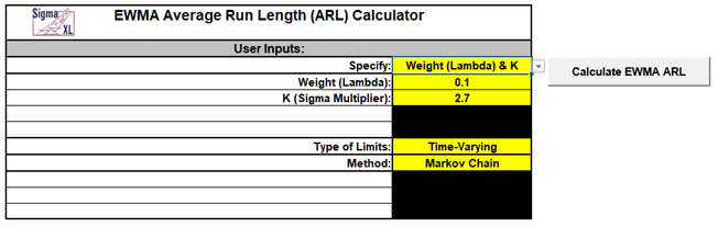
2. The default template settings are Specify = Weight (Lambda) & K, Weight (Lambda) = 0.1, K (Sigma Multiplier) = 2.7, Type of Limits = Time-Varying, Method = Markov Chain.
   
   
   Notes: Parameters to be specified will be shown in yellow highlight, otherwise they are hidden. The EWMA parameter Weight (Lambda) is a value between 0 and 1 and controls the amount of influence that previous observations have on the current EWMA statistic. A value near 1 puts almost all weight on the current observation, making it resemble a Shewhart chart. For values near 0, a small weight is applied to almost all of the past observations, so the EWMA chart performance is similar to that of a CUSUM chart. The EWMA parameter K (Sigma Multiplier) is a value typically between 2 and 4. It is also referred to as L, but SigmaXL uses K to avoid confusion with Lambda.
   
   The EWMA control chart template has hard coded the Type of Limits as Time-Varying, since they improve the sensitivity of the EWMA to detect early changes in the process mean. Fixedis included as an option here for comparison of ARL results to published papers. Also, if the process is in control when the EWMA is started but shifts out of control after the control limits have stabilized, the more appropriate ARL for such a case would be Type of Limits = Fixed.
   
   The Markov Chain approximation is fast and accurate to compute ARLs. Monte Carlo simulation allows you to assess robustness to nonnormality and also produces the table of Run Length Standard Deviation and Percentiles (scroll right to view).
   
   For further details on the Markov Chain approximation see Lucas [1] for fixed and Steiner [3] for time-varying. Monte Carlo simulation uses the Pearson Family of distributions to match the specified skewness and kurtosis.
   
   The EWMA ARL is for a two-sided chart with zero-state, i.e., the shift is assumed to occur at the start. The mean and standard deviation are also assumed to be known. This will not likely be the case in use, but is still useful for determining parameter settings and comparison of ARL across chart types.
   
   All ARL calculations for EWMA use a standardized in-control mean=0 and sigma=1.
   
   
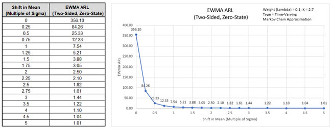
3. Click the Calculate EWMA ARL button to reproduce the ARL table and chart.
   
   
   
   The ARL₀ (in-control ARL with 0 shift in mean) for the EWMA chart with these settings is 356.1, which is close to the Shewhart ARL₀ of 370.4. The ARL₁ for a small 1 sigma shift in mean is 7.54, so is much faster to detect than the ARL₁ of 43.89 for Shewhart Individuals and faster to detect than the Monte Carlo ARL₁ of 9.7 for the Shewhart Individuals with 8 tests for special causes.


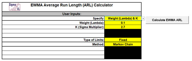
4. Now we will compare time-varying to fixed limits. Select Specify = Weight (Lambda) & K. Enter Weight (Lambda) = 0.1, K (Sigma Multiplier) = 2.7, Type of Limits = Fixed, Method = Markov Chain.
   
   
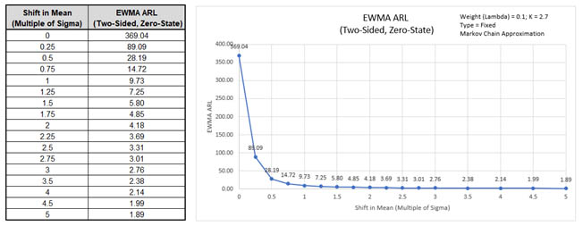
5. Click the Calculate EWMA ARL button to produce the ARL table and chart for these settings:
   
   
   The ARL₀ for the EWMA chart with these settings is 369.04, which is close to the Shewhart ARL₀ of 370.4. The ARL₁ for a small 1 sigma shift in mean with fixed limits is 9.73, which is slower than the ARL₁ with time-varying limits of 7.54.
   
   
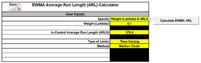
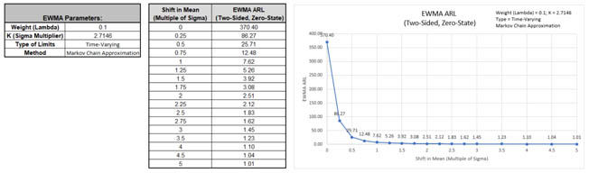
6. Next, we will specify Weight (Lambda) = 0.1, the Shewhart ARL₀ value of 370.4 and solve for the K (Sigma Multiplier). Enter Specify = Weight (Lambda) & ARL0, Weight (Lambda) = 0.1, In-Control Average Run Length (ARL0) = 370.4, Type of Limits = Time-Varying, Method = Markov Chain.
   
   
7. Click the Calculate EWMA ARL button to produce the updated EWMA Parameters, ARL table and chart for these settings:
   
   
   The ARL₀ for the EWMA chart with these settings is 370.4 as specified. The K (Sigma Multiplier) solved to obtain this ARL₀ value is 2.7146. The ARL₁ for a small 1 sigma shift in mean is 7.62.
   
   
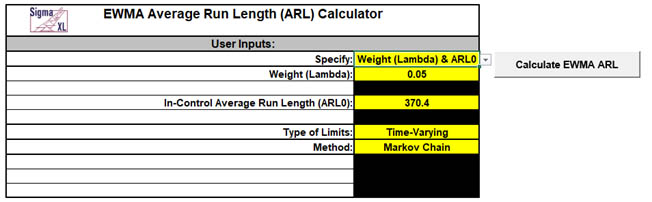
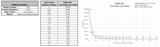
8. Now we will specify Weight (Lambda) = 0.05, the Shewhart ARL₀ value of 370.4 and solve for the K (Sigma Multiplier). Enter Specify = Weight (Lambda) & ARL0, Weight (Lambda) = 0.05, In-Control Average Run Length (ARL0) = 370.4, Type of Limits = Time-Varying, Method = Markov Chain.
   
   
9. Click the Calculate EWMA ARL button to produce the updated EWMA Parameters, ARL table and chart for these settings:
   
   
   The ARL₀ for the EWMA chart with these settings is 370.4 as specified. The K (Sigma Multiplier) solved to obtain this ARL₀ value is 2.523. The ARL1 for a small 1 sigma shift in mean is 6.76.
   
   
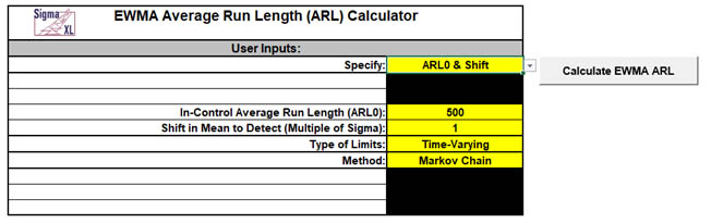
10. Next, we will specify an ARL₀ value of 500 with a desired optimization to detect a 1 sigma shift in mean. The calculator will solve for the optimal Weight (Lambda) and K (Sigma Multiplier). Enter Specify = ARL0 & Shift, In-Control Average Run Length (ARL0) = 500, Shift in Mean to Detect (Multiple of Sigma) = 1, Type of Limits = Time-Varying, Method = Markov Chain.
    
    
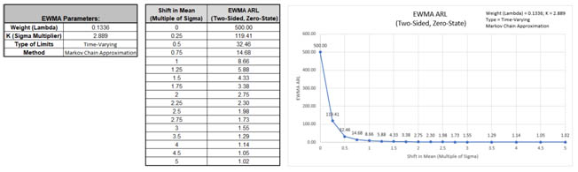
11. Click the Calculate EWMA ARL button to produce the EWMA Parameters, ARL table and chart for these settings:
    
    
    The ARL₀ for the EWMA chart with these settings is 500.0 as specified. The ARL₁ for a small 1 sigma shift in mean is 8.66. The solved parameters are Weight (Lambda) = 0.1336 and K (Sigma Multiplier) = 2.889.
    
    Note: Weight (Lambda) is first solved using fixed limits. This value is then used to solve for K using time-varying limits.
    
    
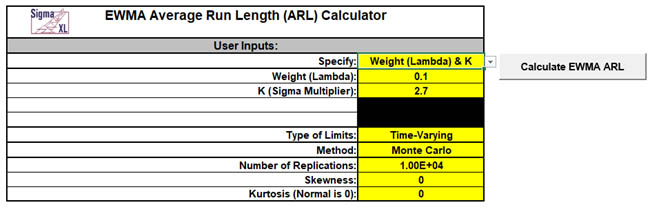
12. Now we will use Monte Carlo simulation to obtain approximate Run Length standard deviation and percentiles. Enter Specify = Weight (Lambda) & K, Weight (Lambda) = 0.1, K (Sigma Multiplier) = 2.7, Type of Limits = Time-Varying, Method = Monte Carlo, Number of Replications = 1e4, Skewness = 0, Kurtosis (Normal is 0) = 0.
    
    
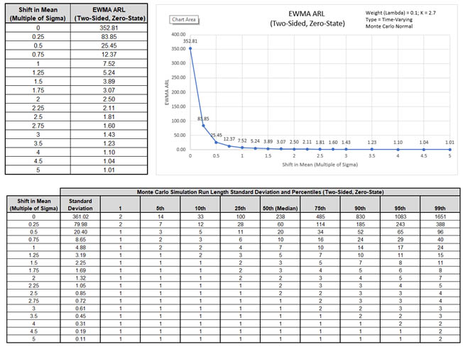
13. Click the Calculate EWMA ARL button to produce the Monte Carlo approximate ARL table, ARL chart and Run Length Standard Deviation and Percentiles table. Monte Carlo simulation with 10,000 (1e4) replications will take about a minute to run.
    
    
    The additional run length statistics show the large variation of run length values. The MRL₀ = 238 (in-control median run length with 0 shift in process mean).
    
    Note: The results will vary slightly since this is Monte Carlo simulation.
    
    
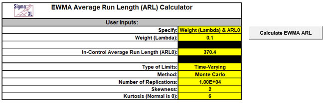
14. We will now assess robustness to nonnormality using Monte Carlo simulation with Weight (Lambda) = 0.1 and a specified ARL₀ of 370.4 for comparison to Shewhart. Enter Specify = Weight (Lambda) & ARL0, Weight (Lambda) = 0.1, In-Control Average Run Length (ARL0) = 370.4, Type of Limits = Time-Varying, Method = Monte Carlo, Number of Replications = 1e4, Skewness = 2, Kurtosis (Normal is 0) = 6.
    
    
    
    Note: The EWMA parameter K (Sigma Multiplier) will be solved using Markov-Chain approximation and assume a Normal distribution, so will match the value previously calculated above (6).
    
    
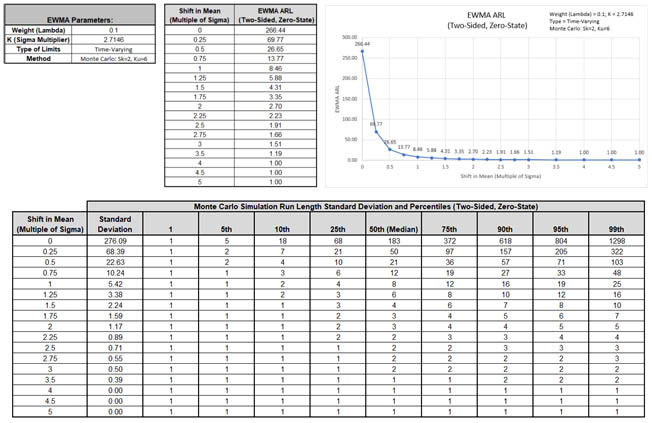
15. Click the Calculate EWMA ARL button to produce the updated EWMA Parameters, Monte Carlo approximate ARL table, ARL chart and Run Length Standard Deviation and Percentiles table:
    
    
    ARL₀ is approximately 266.4 which is a 1.4 x increase (370.4/266.4) in false alarms compared to Normal but is a much better performance than the ARL₀ = 55 result for Shewhart Individuals. MRL₀ is approx. 183.
    
    
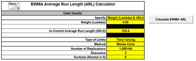
16. Next, we will assess robustness to nonnormality using Monte Carlo simulation with a lower Weight (Lambda) = 0.05 and a specified ARL₀ of 370.4. Enter Specify = Weight (Lambda) & ARL0, Weight (Lambda) = 0.05, In-Control Average Run Length (ARL0) = 370.4, Type of Limits = Time-Varying, Method = Monte Carlo, Number of Replications = 1e4, Skewness = 2, Kurtosis (Normal is 0) = 6.
    
    
    Note: Montgomery [2] (Table 9.12)and Borror, Montgomery &Runger [4] point out that the EWMA becomes more robust with lower values of Lambda.
    
    
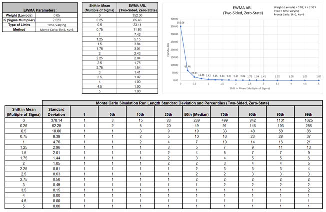
17. Click the Calculate EWMA ARL button to produce the updated EWMA Parameters, Monte Carlo approximate ARL table, ARL chart and Run Length Standard Deviation and Percentiles table:
    
    
    ARL0 is approximately 352 which is close to the original specified 370.4. The MRL0 is approx. 239. If robustness to non-normality is a concern then a Weight (Lambda) = 0.05 is recommended.

1. Specify EWMA parameters: Weight (Lambda) & K, Weight (Lambda) &ARL0 or ARL0& Shift using the drop-down list. Parameters to be specified will be shown in yellow highlight, otherwise they are hidden.
2. If applicable, enter the EWMA parameter Weight (Lambda). This is a value between 0 and 1 and controls the amount of influence that previous observations have on the current EWMA statistic. A value near 1 puts almost all weight on the current observation, making it resemble a Shewhart chart. For values near 0, a small weight is applied to almost all of the past observations, so the EWMA chart performance is similar to that of a CUSUM chart.
3. If applicable, enter the EWMA parameter K (Sigma Multiplier). This is a value typically between 2 and 4. It is also referred to as L, but SigmaXL uses K to avoid confusion with Lambda.
4. If applicable, enter the desired In-Control Average Run Length (ARL0). This will be the target ARL for mean shift = 0 and should be a large value to minimize false alarms, typically 370 to 500. The K (Sigma Multiplier) will be solved to achieve this ARL0, given a specified Weight (Lambda) value.
5. If applicable, enter the desired Shift in Mean to Detect (Multiple of Sigma). The Weight (Lambda) value that minimizes ARL for the specified shift will be solved.
6. Select Type of Limits: Time-Varying or Fixed using the drop-down list.
7. The EWMA control chart template uses time-varying control limits since they improve the sensitivity of the EWMA to detect early changes in the process mean. Published ARL tables typically use fixed limits, so providing both allows comparison between the two types.
8. Select Method: Markov Chain or Monte Carlo using the drop-down list. Markov Chain approximation is fast and accurate to compute ARLs. Monte Carlo simulation allows you to assess robustness to non-normality and also produces the table of Run Length Standard Deviation and Percentiles (scroll right to view).
9. For further details on the Markov Chain approximation see Lucas [1] for fixed and Steiner [3] for time-varying. Monte Carlo simulation uses the Pearson Family of distributions to match the specified skewness and kurtosis.
10. If applicable, enter Number of Replications. 1000 (1e3) replications will be fast, approx. 10 seconds, but will have an ARL0 error approx. = +/- 10%; 10,000 (1e4) replications will take about a minute, with an ARL0 error = +/- 3.2%; 100,000 (1e5) replications will take about ten minutes, with an ARL0 error = +/- 1%.
11. If applicable, enter Skewness. Skewness must be >= 0. Skewness = 0 is symmetric.
12. If applicable, enter Kurtosis (Normal is 0). Also known as Excess Kurtosis, it must be >= Skewness^2 - 1.48. This is required to keep the distribution unimodal. If Skewness=0 and Kurtosis = 0, the distribution is normal.
13. Click the Calculate EWMA ARL button to produce the ARL table and chart. If Monte Carlo was selected, the table of Run Length Standard Deviation and Percentiles will also be produced.
14. The EWMA ARL is for a two-sided chart with zero-state, i.e., the shift is assumed to occur at the start. The mean and standard deviation are also assumed to be known. This will not likely be the case in use, but is still useful for determining parameter settings and comparison of ARL across chart types.
15. Due to the complexity of calculations, SigmaXL must be loaded and appear on the menu in order for this template to function. Do not add or delete rows or columns in this template.

REFERENCES:

1. Lucas J.M. and Saccucci M.S. (1990), “Exponentially weighted moving average control schemes: Properties and enhancements”, Technometrics 32, 1-12.
2. Montgomery, D.C. (2013), Introduction to Statistical Quality Control, Seventh Ed., Wiley.
3. Steiner, S. H. (1999), "EWMA control charts with time-varying control limits and fast initial response", Journal of Quality Technology 31(1), 75-86.
4. Borror, C. M., Montgomery, D.C. and RungerG. C. (1999). “Robustness of the EWMA Control Chartto Nonnormality,” Journal of Quality Technology, 31(3), 309–316.