Include Top

Advanced Multiple Regression with Two-Way Interactions


Click here for more information about Advanced Multiple Regression dialogs and options.

    We will revisit the previous regression analysis of Overall Satisfaction versus Responsive to Calls, Ease of Communications and Customer Type but now, using advanced multiple regression, we will:

    • Standardize the continuous predictors

    • Include two-way interactions

    • Discuss prediction equation with continuous and categorical predictors

    • Assess R-Square Predicted and R-Square K-fold for validation

    • Review the Parameter Estimates and ANOVA for Predictors report with Pareto of Percent Contribution and Pareto of Standardized Effects

    • Review the Durbin-Watson Test for Autocorrelation in Residuals and Breusch-Pagan Test for Constant Variance

    • Examine Residual Plots

    • Look at Main Effects and Interaction Plots with fitted means

    • Use Forward Selection with R-Square Predicted criterion to refine the model

    • Refit the model using Box-Cox Transformation

    • Find optimum values for predictors that maximize Overall Satisfaction

    • Create a Contour and Surface Plot to visualize the relationship of Overall Satisfaction versus Responsive to Calls and Ease of Communications

    • Demonstrate Best Subsets with AICc criterion

    • Demonstrate the use of Test/Withhold Sample ID
  1. Open Customer Data.xlsx. Click Sheet 1 Tab (or press F4 to activate last worksheet). Click SigmaXL > Statistical Tools > Advanced Multiple Regression > Fit Multiple Regression Model. If necessary, click Use Entire Data Table, click Next.

  2. Select Overall Satisfaction, click Numeric Response (Y) >>, select Responsive to Calls and Ease of Communications, click Continuous Predictors (X) >>, select Customer Type, click Categorical Predictors (X) >>. Check Standardize Continuous Predictors with default option Standardize: (Xi - Mean)/StDev. Check Display Regression Equation with Unstandardized Coefficients. We will use the default Coding for Categorical Predictors (1,0). Use the default Confidence Level = 95.0%. Regular Residual Plots are checked by default. Check Main Effects Plots and Interaction Plots. Leave Box-Cox Transformation unchecked for now - this will be used later. We will not use Test/Withhold Sample ID at this time, it will be demonstrated later.

    Multiple Regression Variables

    Tip: If you are planning to include interaction terms in the model, always ensure that Standardize Continuous Predictors is checked. This has two benefits: the predictors are scaled to the same units so coefficients can be meaningfully compared and it dramatically reduces the multicollinearity VIF scores.

    Tip: Check Display Regression Equation with Unstandardized Coefficients to display the prediction equation with unstandardized/uncoded coefficients. This format is easier to interpret with only one coefficient value for each predictor.

  3. Click Advanced Options. Check K-Fold Cross Validation with default Number of Folds (K) = 10 and Seed = 1234. Assume Constant Variance/No AC, Term ANOVA Sum of Squares with Adjusted (Type III), R-Square Pareto Chart, Standardized Effect Pareto Chart are checked by default. Keep Stepwise/Best Subsets Regression unchecked for now - this will be used later. Saturated Model Pseudo Standard Error (Lenth's PSE) is checked by default, but is not used here, as this is only applicable to saturated models with 0 error degrees of freedom.

    Multiple Regression Model

  4. Click OK. Click Next >>.

  5. Using Term Generator, select ME + 2-Way Interactions. Click Select All >>. Include Constant is checked by default.

    Multiple Regression Model

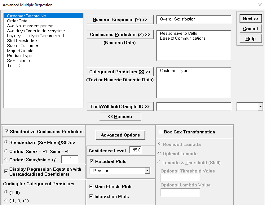
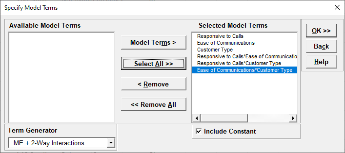
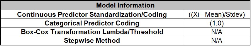
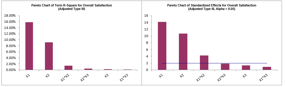
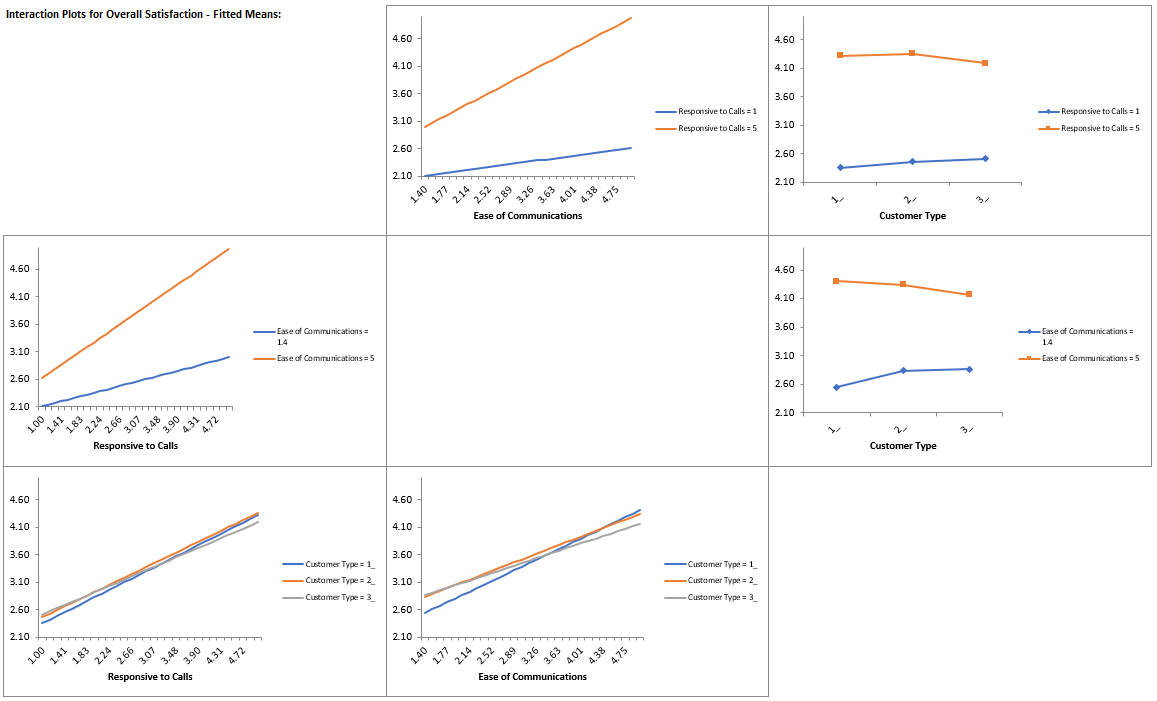
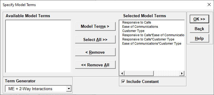
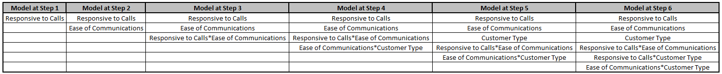
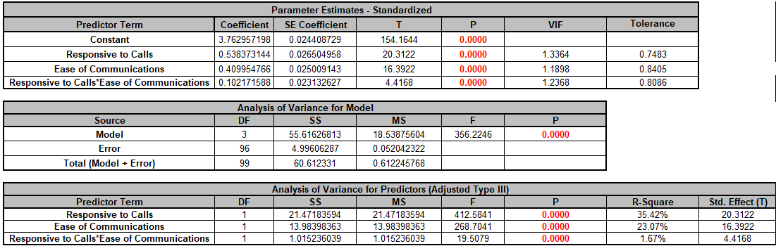
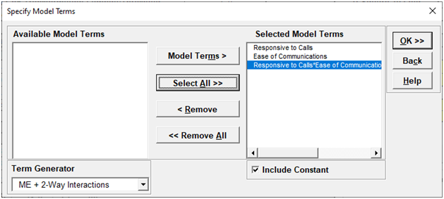
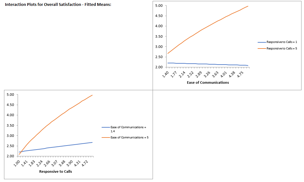
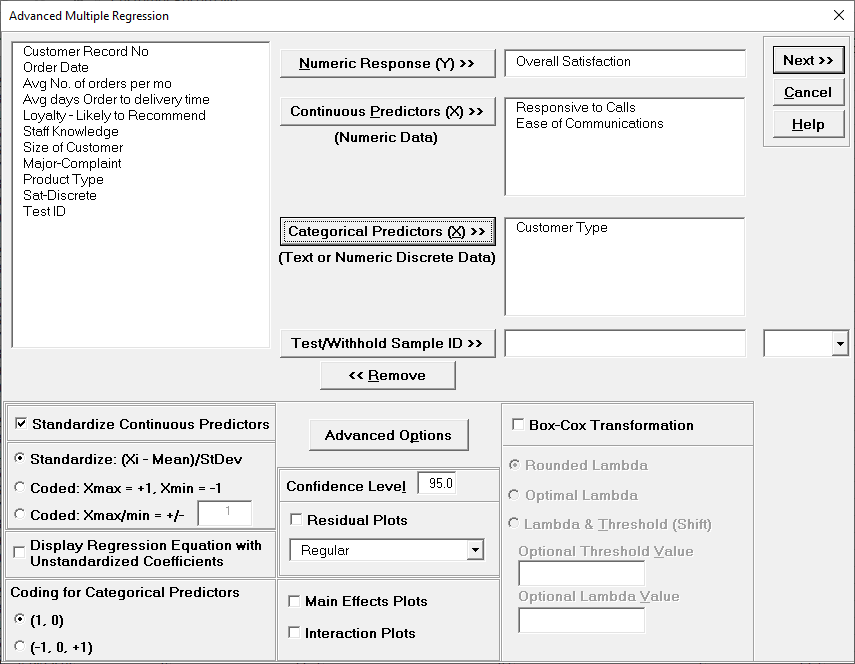
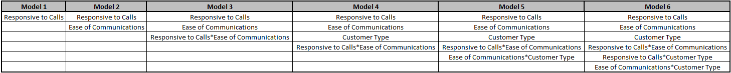
  6. We are adding the three possible 2-way interactions. Note that the three interaction terms are: continuous*continuous, continuous*categorical and continuous*categorical.

  7. Click OK >>. The Advanced Multiple Regression report is given.

  8. The Regression Equation with unstandardized/uncoded coefficients is:

  9. Multiple Regression Model (Uncoded): Overall Satisfaction = (1.38507)
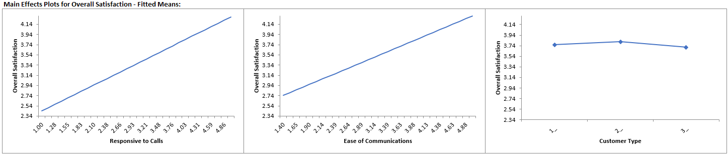
    + (0.111481)*Responsive_to_Calls
    + (0.126645)*Ease_of_Communications
    + (0.505067)*(IF(Customer_Type="2_",1,0))
    + (0.821635)*(IF(Customer_Type="3_",1,0))
    + (0.101385)*Responsive_to_Calls*Ease_of_Communications
    + (-0.0184748)*Responsive_to_Calls*(IF(Customer_Type="2_",1,0))
    + (-0.0728492)*Responsive_to_Calls*(IF(Customer_Type="3_",1,0))
    + (-0.0997064)*Ease_of_Communications*(IF(Customer_Type="2_",1,0))
    + (-0.156844)*Ease_of_Communications*(IF(Customer_Type="3_",1,0))

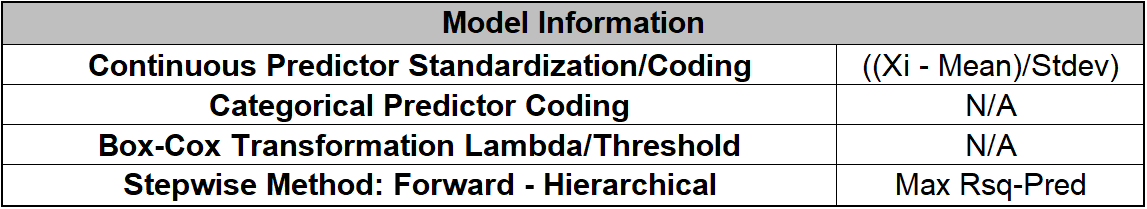
    Note blanks and special characters in the predictor names are converted to the underscore character "_". The numeric Customer Type 1, 2, 3 has also been converted to text so appears as "1_", "2_", "3_", where "1_" is the hidden reference level.

    For categorical predictors, IF statements are used, but exclude the hidden reference level.

    This is the display version of the prediction equation given at cell L14 (which has more precision for the coefficients and predictor names are converted to legal Excel range names by padding with the underscore "_" character). If the equation exceeds 8000 characters (Excel's legal limit for a formula is 8192), then a truncated version is displayed and cell L14 does not show the formula.

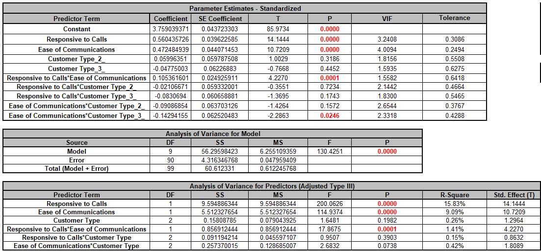
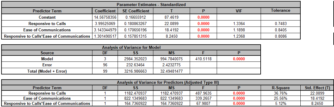
    Note, these coefficients do not match those given in the Parameter Estimates table, since they are Standardized. If consistency is desired, one can always rerun the analysis with Display Regression Equation with Unstandardized Coefficients unchecked.

  10. The Model Summary is:

    Multiple Regression Model

    R-Square = 92.88%, the percent variation explained by the model is quite good. R-Square Adjusted = 92.17%, which includes a penalty for the number of terms in the model design matrix, is also good, and S = 0.2190. These are an improvement over the previous analysis with R-Square = 90.58%, R-Square Adjusted = 90.18% and S = 0.2452, due to the addition of the three interaction terms. R-Square Predicted = 89.88%, also known as Leave-One-Out Cross-Validation, indicates how well a regression model predicts responses for new observations and is typically less than R-Square Adjusted. This is also good.

  11. The Model Information is given as:

    Multiple Regression Model

    This summarizes the selected options for the model and, if applicable, will include Box-Cox Lambda and Threshold values.

  12. The Information Criteria and Validation table is given as:

    Multiple Regression Model

    The information criteria AICc and BIC are reported here, but are used for model comparison. We will revisit these when we do model refinement with Forward Selection. R-Square 10-Fold = 89.54%, the R-Square from K-Fold Cross-Validation is good. It is approximately the same as the R-Square Predicted. S 10-Fold = 0.2518 while slightly higher than S, as expected, is also good. Repeating the analysis with a different K and/or seed will produce slightly different results for R-Square and S K-Fold.

  13. The Parameter Estimates - Standardized, Analysis of Variance for Model, Analysis of Variance for Predictors (Adjusted Type III) tables, Pareto of Term R-Square and Pareto of Standardized Effects are shown:

    Multiple Regression Model

    Multiple Regression Model

    Multiple Regression Model

    The P-Values for continuous predictors are the same in the Parameter Estimates and ANOVA for Predictors tables. For categorical predictors and interactions involving a categorical predictor, the Parameter Estimates table gives a Coefficient and P-Value for each level, excluding the hidden reference level. The ANOVA for Predictors table gives an overall P-Value for each of the categorical terms.

    Customer Type is insignificant as a main effect, but is potentially significant in the Ease of Communications*Customer Type interaction (Term P-Value = .0738).

    The Responsive to Calls*Customer Type interaction is not significant (Term P-Value = 0.3903). However, in this example, we will not use P-Values to decide what terms are removed and what terms remain in the model, rather model refinement will be based on the criterion R-Square Predicted.

    The Pareto Chart of Term R-Square and Pareto Chart of Standardized Effects graphically present the information given in the Predictor ANOVA table and show that Responsive to Calls, Ease of Communications and Responsive to Calls*Ease of Communications are the dominant contributors to the variability in Overall Satisfaction. Note that the Term R-Square values do not add up to R-Square = 92.88%, since these are Type III Adjusted Sum-of-Squares, but they are still useful to assess relative contribution. If we included Type I Adjusted Sum-of-Squares, the Term R-Square values would add up to 92.88%, but have the disadvantage that the individual Term R-Square values depend on model order, whereas Type III do not. If the predictors are orthogonal, then Type III and Type I are the same.

    The Variance Inflation Factor (VIF) scores are all < 5, so acceptable, but they are higher than those we saw in the previous analysis, so this is something that we will want to keep an eye on as we progress with model refinement.

  14. The Durbin-Watson Test for Autocorrelation in Residuals table is:

    Multiple Regression Model

    The Durbin Watson (DW) test is used to detect the presence of positive or negative autocorrelation in the residuals at Lag 1. If either P-Value is < .05, then there is significant autocorrelation.

    This may be evident in the plot of residuals versus observation order. We will look at the residuals plots shortly.

    Note that DW does not test for higher order lags. If that is a concern, then use the Time Series Forecasting tools, particularly the Autocorrelation ACF/PACF Plots on the residuals and model using ARIMA with Predictors.

    Here we do see significant positive autocorrelation, which is a problem because it violates the regression assumption of independence.

    Tip: Note that this status may change with model refinement, as we will see this is the case in this example. If after model refinement, the Durbin Watson test still shows significant autocorrelation, then refit the model using Recall Last Dialog, click Advanced Options in the Advanced Multiple Regression dialog, and uncheck Assume Constant Variance/No AC. SigmaXL will apply the Newey-West (Lag 1) robust standard errors for non-constant variance with autocorrelation. For details, see the SigmaXL workbook Appendix: Advanced Multiple Regression.

  15. The Breusch-Pagan Test for Constant Variance is:

    Multiple Regression Model

    There are two versions of the Breusch-Pagan (BP) test for Constant Variance: Normal and Koenker Studentized - Robust. SigmaXL applies an Anderson-Darling Normality test to the residuals in order to automatically select which version to use. If the AD P-Value < 0.05, Koenker Studentized - Robust is used.

    The report includes the test for All Terms and for individual predictors. All Terms denotes that all terms are in the model. This should be used to decide whether or not to take corrective action. The individual predictor terms are evaluated one-at-a-time and provide supplementary information for diagnostic purposes. Note, this should always be used in conjunction with an examination of the residual plots.

    Here we see that the All Terms test is not significant, but the Responsive to Calls*Customer Type interaction is significant.

    Tip: As with the Durbin-Watson test, this status may change with model refinement. If the All Terms test is significant after model refinement, including a Box-Cox transformation, then refit the model using Recall Last Dialog, click Advanced Options in the Advanced Multiple Regression dialog, and uncheck Assume Constant Variance/No AC. SigmaXL will apply the White robust standard errors for non-constant variance. For details, see the SigmaXL workbook Appendix: Advanced Multiple Regression.

    Tip: Lack of Constant Variance (a.k.a. Heteroskedasticity) is a nuisance for regression modelling but is also an opportunity. Examining the residual plots and BP individual predictors may yield process knowledge that identifies variance reduction opportunities.

  16. Scroll to the Predicted Response Calculator. Enter Responsive to Calls and Ease of Communication values = 5 and select Customer Type = 2_ from the dropdown list to predict Overall Satisfaction including the 95% confidence interval for the long term mean and 95% prediction interval for individual values:

    Multiple Regression Model

    The use of a dropdown list for categorical predictors is easier than having to enter coded 0,1 values.

  17. Click on Sheet MReg1 - Residuals to view the Residual Plots. Note, Sheet MReg# will increment every time a model is refitted.

    Multiple Regression Model
    Multiple Regression Model

    Regular Residual Plots display the raw residuals (Y - Ŷ), the unexplained variation from the regression model, with a Histogram, Normal Probability Plot, Residuals vs Data Order, Residuals vs Predicted Values, Residuals vs Continuous Predictors and Residuals vs Categorical Predictors.

    We expect to see the residuals normally distributed with no obvious patterns in the above graphs. This is not the case here, but they are better than the residual plots in the previous analysis, which showed a strong trend in the Residuals versus Predicted Values.

    The table of Residuals, Standardized Residuals, Studentized (Deleted t) Residuals, Cook's Distance (Influence), Leverage and DFITS are given to the left of the Residual Plots:

    Multiple Regression Table of Residuals

    Standardized Residuals are the residuals, divided by an estimate of its standard deviation. This makes it easier to detect outliers. Standardized residuals greater than 3 and less than -3 are considered outliers and highlighted in red. Standardized residuals for observation numbers 43, 66 and 76 are highlighted. Excel’s filter by Font Color can be used to view just the outliers:

    Standardized Residuals

    Note that this filter action will cause the Residual Plots to be hidden; clear the Filter to view the Residual Plots again.

    Studentized (Deleted t) Residuals are computed in the same way that standardized residuals are, except that the ith observation is removed before performing the regression fit. This prevents the ith observation from influencing the regression model, resulting in unusual observations being more likely to stand out.

    Leverage is a measure of how far an individual X predictor value deviates from its mean. High leverage points can potentially have a strong effect on the estimate of regression coefficients. Leverage values fall between 0 and 1.

    Cook's distance and DFITS are overall measures of influence. An observation is said to be influential if removing the observation substantially changes the estimate of model coefficients. Cook’s distance can be thought of as the product of leverage and the standardized residual squared; DFITS as the product of leverage and the studentized residual. These diagnostic measures can be manually plotted using a Run Chart to identify unusually large values.

    Commonly used rough criterion/cutoff for Cook’s distance are: > 0.5, potentially influential and > 1, likely influential. A more accurate cutoff is the median of the F distribution: >F(0.5,p,n-p), where n is the sample size and p is the number of terms in the model design matrix, including the constant (i.e., the number of rows in the Parameter Estimates table). So in this example using the Excel formula, the cutoff is: =F.DIST(0.5, 10,(100-10),TRUE) = 0.114. Excel’s filter > 0.114 can be used to view influential observations based on Cook’s Distance:

    Cook’s Distance Residuals

    Note that this filter action will cause the Residual Plots to be hidden; clear the Filter to view the Residual Plots again.

    A commonly used criterion for absolute value of DFITS is >2√(p/n). So in this example,
    |DFITS| > 2√(10/100) = 0.632.

    An observation that is an outlier and influential should be examined for measurement error or possible assignable cause. Observation 43 is clearly the most influential outlier, so you could try refitting the model excluding that observation to assess the influence. This would need to be done manually, but we will not do that in this demonstration.

    The table to the right of the Residual Plots is the stored model design matrix with residuals. This can be used to manually create additional residual plots (use SigmaXL > Graphical Tools > Scatter Plots) for residuals versus interaction terms:

    residuals versus interaction terms

  18. Click on Sheet MReg1 - Plots. The Main Effects Plots and Interaction Plots for Overall Satisfaction are shown. These are based on Fitted Means as predicted by the model, not Data Means (as used in SigmaXL's Design of Experiments).

    Multiple Regression Model

    Main Effects Plots with Fitted Means use the predicted value for the response versus input predictor value, while holding all other variables constant. Continuous are held at their respective means and categorical are weighted equally.

    Here we see that Responsive to Calls has the steepest slope followed by Ease of Communications. Customer Type does not appear to be an important factor, however, we also need to consider the interaction plots:

    Multiple Regression Model

    As with Main Effects Plots for Fitted Means, all continuous predictors not being plotted are held at their respective means and categorical are weighted equally.

    Here we can clearly see a moderate interaction effect with the different slopes in Responsive to Calls*Ease of Communications, i.e., the effect that Responsive to Calls has on Overall Satisfaction depends on the value of Ease of Communications. Similarly, the effect that Ease of Communications has on Overall Satisfaction depends on the value of Responsive to Calls.

    There also appears to be a slight interaction effect with the different slopes in Customer Type by Ease of Communications.

    These plots should always be used in conjunction with the above Parameter Estimates table and Pareto Charts to determine significance.

    Note, if an interaction term is not in the model, the interaction plot is still displayed, but it is shaded grey.

  19. Click Recall Last Dialog (or press F3). Click Advanced Options in the Advanced Multiple Regression dialog.

  20. Check Stepwise/Best Subsets Regression. Select Forward Selection and Criterion: R-Square Predicted. Hierarchical is checked by default.

    Multiple Regression Model

  21. Click OK. Click Next >>.

    Multiple Regression Model

  22. Click OK >>.

  23. Click on Sheet MReg2 - Report. Note, Sheet MReg# will increment every time a model is refitted. The Forward Selection report is given:

    Multiple Regression Model

    Multiple Regression Model

    Multiple Regression Model

    Scroll across to view the report tables. Forward Selection identifies the model at Step 3 (denoted with double asterisk ** and highlighted in yellow), as having the largest R-Square Predicted value = 90.35%. ** R-Sq(Pred)** denotes that this is the criterion used to select the final model.

    Note that while the model at Step 4 has a slightly higher R-Square Predicted, it is not selected because it does not include Customer Type, which is needed for the model to be Hierarchical. When Customer Type is added at Step 5, the R-Square Predicted value is less than that of Step 3.

    Mode can be Add, Add_H, or Remove. Add_H denotes a predictor being added for Hierarchy. Remove is not applicable for Forward Selection.

    # Predictors is the number of continuous or categorical predictors in the model, excluding the constant.

    # Model Terms is the number of columns in the model design matrix, including the constant and coded columns for categorical predictors. This is the value used by all of the metrics.

    P is the P-Value for the predictor. This is the P-Value for the term at that particular step and is subject to change when other terms are added. P-Values are used for model selection (i.e., stopping rule) only when Alpha-to-Enter has been specified. Since we selected Criterion, they are not used for model selection, but the decision of what term to consider at a particular step is still based on the P-Value.

    S is the model standard deviation or root-mean-square error at that step.

    R-Sq is the R-Square, i.e., the percent variation in response that is explained by the model at that step.

    R-Sq(Adj) is the R-Square Adjusted for the model at that step. The model at Step 5 has the maximum R-Square Adjusted = 92.18%.

    R-Sq(Pred) is the R-Square Predicted for the model at that step.

    R-Sq(10-Fold), R-Square K-Fold, is reported only if it is selected as the criterion.

    PRESS is the prediction error sum of squares and is used to calculate R-Square Predicted.

    AICc is the Akaike Information Criterion corrected for small sample sizes. If we had selected AICc as the criterion, then the model at Step 5 would have been selected with minimum AICc = -8.3976 (Step 4 is excluded due to the Hiearchical requirement).

    BIC is the Bayesian Information Criterion and includes a stronger penalty for the number of terms in the model design matrix. The model at Step 3 has the minimum BIC = 7.1616.

    Mallows' Cp is a measure that compares the full model to candidate models and is similar to the Akaike Information Criterion. An unbiased model has the Mallows' Cp close to the number of model terms. Mallows' Cp for the model with all terms will exactly match the number of model terms, which in this example is 10. The model with optimal Mallows' Cp value for this example is at Step 5, Mallows' Cp = 7.9015, which is close to the # Model Terms = 8.

    Condition # measures whether a model is well conditioned. An ill conditioned model will have a large change in coefficient values for a small change in the input data. A rule of thumb is that CN > 100 indicates moderate multicollinearity, so all of the models considered here have an acceptable condition number.

    For details on these metrics, see the SigmaXL workbook Appendix: Advanced Multiple Regression.

    In conclusion, we could use either Step 3 or Step 5 as our final model, but we will proceed with the simpler model at Step 3. It may be beneficial to refit using a different criterion for Forward such as AICc or BIC and/or a different method. Later, we will demonstrate the use of Best Subsets with the AICc criterion.

  24. Click on Sheet MReg2 - Model Overall

  25. The Model Summary is:

    Multiple Regression Model

    R-Square = 91.76% and R-Square Adjusted = 91.5% have been reduced slightly (versus the full model R-Square = 92.88% and R-Square Adjusted = 92.17%). S = 0.2281 is slightly higher than the full model S = 0.219. However, R-Square Predicted = 90.35% is an improvement over the full model R-Square Predicted = 89.88% and we have simplified the model by removing all terms with Customer Type. This will make interpretation much easier.

  26. The Model Information is given as:

    Multiple Regression Model

    This summarizes the selected options for the model showing that the Stepwise Method is Forward Selection, Hierarchical and the Criterion is Max Rsq-Pred, Maximize R-Square Predicted.

  27. The Information Criteria and Validation table is given as:

    Multiple Regression Model

    R-Square 10-Fold = 90.07% is an improvement over the full model R-Square 10-Fold = 89.54%. S 10-Fold = 0.2453 is slightly less than the full model S 10-Fold = 0.2518.

  28. The Parameter Estimates - Standardized, Analysis of Variance for Model, Analysis of Variance for Predictors (Adjusted Type III) tables, Pareto of Term R-Square and Pareto of Standardized Effects are shown:

    Multiple Regression Model

    Multiple Regression Model

    Multiple Regression Model

    The continuous predictors Responsive to Calls, Ease of Communications and interaction Responsive to Calls*Ease of Communications all show as clearly significant.

    The Pareto Chart of Term R-Square and Pareto Chart of Standardized Effects graphically present the information given in the Predictor ANOVA table and show that main effects Responsive to Calls, Ease of Communications are the dominant contributors to the variability in Overall Satisfaction. The interaction term Responsive to Calls*Ease of Communications is a smaller contributor, but still significant.

    The Variance Inflation Factor (VIF) scores have been reduced from the full model, for example, Ease of Communications VIF = 1.19 versus the full model VIF = 4.01.

  29. The Durbin-Watson Test for Autocorrelation in Residuals table is:

    Multiple Regression Model

    Here, there is no significant positive or negative autocorrelation.

    Note that this is a change from the Durbin Watson Test for the full model which was:

    Multiple Regression Model

    This shows that the Residual diagnostics can change as the model changes with model refinement.

  30. The Breusch-Pagan Test for Constant Variance is:

    Multiple Regression Model

    Here we see that the All Terms test is significant and that the Responsive to Calls*Ease of Communications interaction is also significant. This has changed from the full model which showed that All Terms was not significant:

    Multiple Regression Model

    Next, we will refit the model using a Box-Cox Transformation in order to deal with this violation of the regression assumption of constant variance.

  31. Click Recall Last Dialog (or press F3). Select Customer Type and click << Remove. Uncheck Display Regression Equation with Unstandardized Coefficients. Check Box-Cox Transformation with Rounded Lambda option.

    Multiple Regression Model

  32. Click Advanced Options. Uncheck Stepwise/Best Subsets Regression.

    Multiple Regression Model

    Note, Box-Cox Transformation can be used with Stepwise/Best Subsets Regression but here we want to manually specify the model.

  33. Click OK. Click Next >>. Select ME + 2-Way Interactions. Click Select All >>.

    Multiple Regression Model

  34. Click OK >>. The Advanced Multiple Regression report is given for the revised model. Note that the Model Summary, Information Criteria and Validation, Parameter Estimates, ANOVA, DW and BP Tests, and Residuals are for the Box-Cox transformed response. The Main Effects and Interaction Plots, Predicted Response Calculator, Optimize and Contour/Surface Plots all use an inverse transformation to return to the original units.

  35. The Regression Equation with standardized coefficients is:

    Multiple Regression Model: Overall Satisfaction = ( (14.5676)
    + (3.99525)*((Responsive_to_Calls-3.8644)/1.14029)
    + (3.14334)*((Ease_of_Communications-3.7481)/0.911361)
    + (1.30149)*((Responsive_to_Calls-3.8644)/1.14029)*((Ease_of_Communications-3.7481)/0.911361))^(1/2)

    This is the display version of the prediction equation given at cell L14(which has more precision for the coefficients).

    Note, these coefficients match those given in the Parameter Estimates table since they are standardized. If a simpler form of the prediction equation is desired, one can always rerun the analysis with Display Regression Equation with Unstandardized Coefficients checked.

  36. The Model Summary is:

    Multiple Regression Model

    R-Square, R-Square Adjusted and R-Square Predicted have all increased over the previous untransformed model:

    Multiple Regression Model

    Note that the S = 1.5567 is reported for the Box-Cox Transformed response, so cannot be compared to the untransformed S = 0.2281, but the R-Square statistics can be compared.

  37. The Model Information is given as:

    Multiple Regression Model

    This summarizes the selected options for the model showing the Box-Cox Lambda value = 2 (i.e., the response values are squared) and Stepwise is not used.

  38. The Information Criteria and Validation table is given as:

    Multiple Regression Model

    R-Square 10-Fold has increased over the previous untransformed model:

    Multiple Regression Model

    As noted above, the S 10-Fold = 1.6228 is reported for the Box-Cox Transformed response, so cannot be compared to the untransformed S 10-Fold = 0.2453, but the R-Square 10-Fold statistic can be compared.

  39. The Parameter Estimates - Standardized, Analysis of Variance for Model, Analysis of Variance for Predictors (Adjusted Type III) tables, Pareto of Term R-Square and Pareto of Standardized Effects are shown:

    Multiple Regression Model

    Multiple Regression Model

    Multiple Regression Model

    The interaction Responsive to Calls*Ease of Communications has increased in R-Square % and Standardized Effect versus the untransformed model, so is a stronger interaction effect.

  40. Scroll down to view the Durbin-Watson Test for Autocorrelation in Residuals table:

    Multiple Regression Model

    The DW values have changed slightly from the untransformed model but still shows no significant autocorrelation.

  41. The Breusch-Pagan Test for Constant Variance is:

    Multiple Regression Model

    This is a dramatic change for the BP Test for Constant Variance. The All Terms test now shows as insignificant, as well the Responsive to Calls*Ease of Communications interaction is insignificant. Recall that for the untransformed model, the BP Test was:

    Multiple Regression Model

    Tip: The use of the Box-Cox Transformation has eliminated the problem of non-constant variance in the model. Had that not been the case, we would have then proceeded to refit the model with Assume Constant Variance/No AC unchecked.

    A review of the Residual Plots in Sheet MReg3 - Residuals shows that they still do not exhibit the properties of normally distributed, with no patterns and no outliers, so while not ideal, we will consider this as our final model for the purposes of this demonstration.

  42. Click on Sheet MReg3 - Plots. Note, Sheet MReg# will increment every time a model is refitted. The Main Effects Plots and Interaction Plots for Overall Satisfaction are shown. These are based on Fitted Means as predicted by the model.

    Multiple Regression Model

    Here we see that Responsive to Calls has the steepest slope but now there is some curvature due to the Box-Cox transformation.

    Multiple Regression Model

    We also see the curvature due to the Box-Cox Transformation in the Interaction Plots.

    Here we can clearly see a strong interaction effect with the different slopes in Responsive to Calls*Ease of Communications, i.e., the effect that Responsive to Calls has on Overall Satisfaction depends on the value of Ease of Communications. Similarly, the effect that Ease of Communications has on Overall Satisfaction depends on the value of Responsive to Calls.

  43. Click on Sheet MReg3 - Model. Scroll to the Predicted Response Calculator. Enter Responsive to Calls and Ease of Communication values = 5 to predict Overall Satisfaction with the 95% confidence interval for the long term mean and 95% prediction interval for individual values:

    Multiple Regression Model

    Note the formula at cell L14 is an Excel formula (if the formula exceeds Excel's limit of 8192 characters, it is not given, but a predicted response value is still computed). Since we are applying an inverse transformation to the Box-Cox transformed prediction, the Confidence and Prediction Intervals are not symmetric.

  44. Next, we will use SigmaXL's built in Optimizer. Scroll to view the Optimize Options:

    Multiple Regression Model

    Here we can constrain the continuous predictors, and if there was a categorical predictor, specify a level to use for optimization. If a continuous predictor is integer, change the Integer 0 to 1, and the Optimizer will return only integer values for that predictor.

    We will leave the Optimize Option settings as is.

  45. Scroll back to view the Goal setting and Optimize button. Select Goal = Maximize.

    Multiple Regression Model

    The optimizer uses Multistart Nelder-Mead Simplex to solve for the desired response goal with given constraints. For more information see the SigmaXL workbook Appendix: Single Response Optimization.

  46. Click Optimize. The response solution and prompt to paste values into the Input Settings of the Predicted Response Calculator is given:

    Multiple Regression Model

  47. Click Yes to paste the values.

    Multiple Regression Model

    This confirms that our manual settings were correct to provide the maximum Overall Satisfaction.

  48. Next, we will create a Contour/Surface Plot. Click the Contour/Surface Plots button. Note this button is not available if there are fewer than two continuous predictors.

  49. A new sheet is created, MReg3 - Contour that displays the plots:

    Multiple Regression Model

    The curvature in the response is due to the two-way interaction (and the Box-Cox transformation). We clearly see that maximizing both Response to Calls and Ease of Communications is necessary to maximize Overall Satisfaction.

    The table with the Hold Values, gives the values used to hold a predictor constant if it is not in the plot, so is not applicable here with only one plot based on the two continuous predictors.

    Tip: These values are obtained from the Predicted Response Calculator settings, so if you wish to use different Hold Values, simply select the Model sheet, change the Enter Settings values and recreate the plots.

  50. Next, we will demonstrate the use of Best Subsets Regression. Click Recall Last Dialog (or press F3). Select Customer Type and click Categorical Predictors (X) >>. Uncheck Box-Cox Transformation so that we can compare the Best Subsets report to the earlier Forward Selection report. Uncheck Residual Plots, Main Effects and Interaction Plots as we will not revisit these.

    Multiple Regression Model

  51. Click Advanced Options. Check Stepwise/Best Subsets Regression. Select Best Subsets with default 1 For Each # Pred, Max Time (sec) = 300 and Criterion as AICc. Hierarchical is checked by default.

    Multiple Regression Model

  52. Click OK. Click Next >>. Select ME + 2-Way Interactions, click Select All >>.

    Multiple Regression Model

  53. Click OK >>.

  54. Click on Sheet MReg4 Report. Note, Sheet MReg# will increment every time a model is refitted. The Best Subsets report is given:

    Multiple Regression Model

    Multiple Regression Model

    Multiple Regression Model

    This is similar to the Forward Selection report but instead of steps, shows the "best" model that minimizes the criterion AICc for each number of predictors. The double asterisk ** and yellow highlight show the selected overall best model. Model 5 has the minimum AICc.

    Model 3 has the minimum BIC, but refitting the model with the BIC criterion may result in different models being selected for each # predictors, so it may be beneficial to run Best Subsets twice. We will not do that in this demonstration.

    Note that Best Subsets evaluates only models that satisfy Hierarchy, those that do not are not considered. This simplifies the interpretation of the report.

    R-Square Predicted and R-Square 10-Fold cannot be specified as criterion in Best Subsets due to their computation times, but they are reported here.

    Mode and P given in the Forward Selection report are not applicable for Best Subsets.

  55. Finally, we will demonstrate the use of Test/Withhold Sample ID. This splits the data into a training and test/withhold sample for validation. For this demonstration, we will use the TestID column given in Customer Data.xlsx, but a column of random 0/1 values can also be created manually using the Excel function =IF(RAND()<=0.3,1,0), where 0.3 is the fraction desired for the test/withhold sample, 0 denotes training data, and 1 denotes test data. If this is used, be sure to copy/paste values to freeze the random 0/1 numbers, since RAND is a volatile function which will recalculate every time Excel recalculates. The use of Test/Withhold Sample ID should be with large datasets, so while N=100 doesn’t really qualify as large, we will use this for demonstration purposes and continuity in the example.

  56. Click Recall Last Dialog (or press F3). Select Customer Type and click << Remove. Select Test ID and click Test/Withhold Sample ID >>. We will use the default combo drop down selection = 1, which is used to specify what rows are assigned to the test/withhold sample. Check Box-Cox Transformation with Rounded Lambda option.

    Multiple Regression Dialogue Test/Sample ID

  57. Click Advanced Options. Uncheck Stepwise/Best Subsets Regression.

    Multiple Regression Dialogue Test/Sample ID Advanced Options

    Test/Withhold Sample ID and Box-Cox Transformation can be used with Stepwise/Best Subsets Regression but here we want to manually specify the model.

  58. Click OK. Click Next >>. Select ME + 2-Way Interactions. Click Select All >>.

    Multiple Regression Dialogue Test/Sample ID Terms

  59. Click OK >>. The Test/Withhold Sample report is shown along with the Information Criteria and Validation.

  60. Test/Withhold Sample report

    ID/Column Level indicates what text or numeric value in the Test ID column is used to specify the test sample. Test Sample % shows that the test sample comprises 34% of the data. R-Square Test = 92.65% and S Test = 1.365 are quite good, but note that they will vary if a different random Test ID is used.

  61. Click on Sheet MReg5 – Test.Note, Sheet MReg# will increment every time a model is refitted. The detailed Test report is given:

    Detailed Test report a

    Detailed Test report a

    This gives the Obs. No. (Observation Number) for the Test/Withhold Sample data along with the predictor values, response values, Predicted Response, SE, CI, PI and Box-Cox Transformed Residuals. Residual plots are not provided but they can be created manually using SigmaXL’s graphical tools.

    Tip: If a row specified in the Test/Withhold Sample does not include a response value, it will still appear in this report with the Predicted Response, SE, CI and PI values given. It would be excluded from the Test Sample %, R-Square Test and S Test results.

Advanced Multiple Regression Dialogs and Options

< Back to top

Fit Multiple Regression Model Dialog

Multiple Regression Model

  • Numeric Response- select the response variable. Only one response may be selected at a time, but use Recall SigmaXL Dialog or Press F3 to repeat an analysis with different options or to select a different response. The regression reports will be created on sheets MReg1 - Model Y1name, MReg2 - Model Y2name, etc., but truncated to fit the 31-character limit for Excel sheet names.

  • Continuous Predictors-select continuous numeric predictors. Selections with data as text are error trapped. Note that the character "*" cannot be in the predictor name as this is used to denote a cross product term and will be error trapped.

  • Categorical Predictors - select categorical predictors. Numeric predictors can be used but they will be converted to text and an underscore "_" will be appended to the number. If there are more than 50 unique levels, a warning message is given. Typically, this occurs when the user has incorrectly selected a continuous predictor as categorical.
  • Test/Withhold Sample ID splits the data into a training and test/withhold sample for validation. To create a Test ID column with random 0/1 values, use the Excel function =IF(RAND()<=0.3,1,0), where 0.3 is the fraction desired for the test/withhold sample, 0 denotes training data, and 1 denotes test data. (Be sure to copy/paste values to freeze the random 0/1 numbers). The combo drop down is used to specify what rows are assigned to the test/withhold sample. Note, if a response value is missing from the test/withhold sample, a predicted response value will still be given in the Test report. Use of Test/Withhold Sample ID is recommended for large datasets (N >= 1000).

  • Standardize Continuous Predictors with Standardize: (Yi - Mean)/Stdev will convert continuous predictors to Z-scores. This has two benefits: the predictors are scaled to the same units so coefficients can be meaningfully compared and it dramatically reduces the multicollinearity VIF scores when interactions and/or quadratic terms are specified.

  • Standardize Continuous Predictors with Coded: Ymax = +1, Ymin = -1 scales the continuous predictors so that Ymax is set to +1 and Ymin is set to -1. This is particularly useful for analyzing data from a full or fractional-factorial design of experiments.

  • Standardize Continuous Predictors with Coded: Ymax/Ymin = +/- value scales the continuous predictors so that Ymax is set to +value and Ymin is set to-value. This is particularly useful if one is analyzing data from a response surface design of experiments, where value is set to the alpha axial value such as 1.414 for a two-factor rotatable design.

  • Display Regression Equation with Unstandardized Coefficients displays the prediction equation with unstandardized/uncoded coefficients but the Parameter Estimates table will still show the standardized coefficients. This format is easier to interpret since there is only one coefficient value for each predictor.

  • Coding for Categorical Predictors (1,0) is the standard dummy coding used for categorical predictors, with the hidden reference value being the first alpha-numerically sorted level.

  • Coding for Categorical Predictors (-1,0,+1) is a coding scheme suitable for categorical predictors when the continuous predictors are Coded: Ymax = +1, Ymin = -1. For two levels, the coefficients are magnitude consistent with the continuous predictors. The hidden reference level is the last alpha-numerically sorted level.

  • Confidence Level is used to determine what alpha value is used to highlight P-Values in red, the significance reference line in the Pareto Chart of Standardized Effects, and the percent confidence and prediction interval used in the Predicted Response Calculator.

  • Residual Plots Regular display the raw residuals (Y - Ŷ) with a Histogram, Normal Probability Plot, Residuals vs Data Order, Residuals vs Predicted Values, Residuals vs Continuous Predictors and Residuals vs Categorical Predictors.

  • Residual Plots Standardized display the residuals, divided by an estimate of its standard deviation. This makes it easier to detect outliers. Standardized residuals greater than 3 and less than -3 are considered large (these outliers are highlighted in red).

  • Residual Plots Studentized (Deleted t) display studentized deleted residuals which are computed in the same way that standardized residuals are, except that the ith observation is removed before performing the regression fit. This prevents the ith observation from influencing the regression model, resulting in unusual observations being more likely to stand out.

  • The Residuals report is provided on a separate sheet and includes a table with all residual types to the left of the plots. Other diagnostic measures included, but not plotted are: Cook's Distance (Influence), Leverage and DFITS. Leverage is a measure of how far an individual X predictor value deviates from its mean. High leverage points can potentially have a strong effect on the estimate of regression coefficients. Leverage values fall between 0 and 1. Cook's distance and DFITS are overall measures of influence. An observation is said to be influential if removing the observation substantially changes the estimate of model coefficients. Cook's distance can be thought of as the product of leverage and the standardized residual squared; DFITS as the product of leverage and the studentized residual. These diagnostic measures can be manually plotted using a Run Chart to identify unusually large values. Commonly used rough cutoff criterion for Cook's distance are: > 0.5, potentially influential and > 1, likely influential. A more accurate cutoff is the median of the F distribution: >F(0.5,p,n-p), where n is the sample size and p is the number of terms in the model design matrix, including the constant. A commonly used cutoff criterion for the absolute value of DFITS is: >2√(p/n). An observation that is an outlier and influential should be examined for measurement error or possible assignable cause. You could also try refitting the model excluding that observation to assess the influence.

  • The Residuals report also includes a table to the right of the plots with the stored model design matrix and residuals. This can be used to manually create additional residual plots such as residuals versus interaction or quadratic terms.

  • Tip: For large datsets (> 1K) you may want to uncheck the Residual Plots in order to speed up the analysis.

  • Main Effects Plots and Interaction Plots use fitted means, not data means. If an interaction term is not in the model, the interaction plot is still displayed, but it is shaded grey.

  • Box-Cox Transformation with Rounded Lambda will solve for an optimal lambda and is rounded to the nearest value of: -5, -4, -3, -2, -1, -0.5, 0, 0.5, 1, 2, 3, 4, 5.0 denotes a Ln(Y) transformation, 0.5 is the SQRT(Y), and 1 is untransformed. Threshold (Shift) is computed automatically if the response data includes 0 or negative values, otherwise it is 0. Note that the threshold is subtracted from the data so the value will be negative in order to provide positive response values. Solving lambda is also supported in Stepwise Regression. The reported Parameter Estimates, Model Summary, Information Criteria, Validation, Test Statistics and Residuals are for the Box-Cox transformed response. The Predicted Response Calculator automatically applies an inverse transformation so that the predicted response, confidence and prediction intervals are given in the original untransformed units. Note, Lambda is solved to normalize the regression residuals, not the raw data. It is solved using the classical Box-Cox formula but the actual transformation uses a simple power transformation.

  • Box-Cox Transformation with Optimal Lambda uses the range of -5 to +5 for Lambda. Threshold is computed automatically if the response data includes 0 or negative values.

  • Box-Cox Transformation with Lambda & Threshold (Shift) allows the user to specify Lambda and Threshold. Threshold is typically 0, but if the response data includes 0 or negative values, a negative threshold value should be entered, such that when subtracted from the data, results in positive response values.
Advanced Multiple Regression Options Dialog

Multiple Regression Model

  • Assume Constant Variance/No AC (no autocorrelation in the residuals), if unchecked, SigmaXL will use either White robust standard errors for non-constant variance or Newey-West robust standard errors for non-constant variance with autocorrelation. If either of the Durbin-Watson P-Values are < .05 (i.e., significant positive or negative autocorrelation), Newey-West for Lag 1 is used, otherwise White HC3 is used. This will affect SE Coefficients, P-Values, ANOVA F and P-Values, and Prediction CI/PI. ANOVA F and P-Values are Wald estimates. ANOVA SS Type I Table and Pareto Charts are not available. Note: Stepwise P-Values are not adjusted.

  • Term ANOVA Sum of Squares with Adjusted (Type III) provides a detailed ANOVA table for continuous and categorical predictors. Adjusted Type III is the reduction in the error sum of squares (SS) when the term is added to a model that contains all the remaining terms. Note, categorical terms are considered as a group, unlike the parameter estimates table which uses coding.

  • Term ANOVA Sum of Squares with Sequential (Type I) provides a detailed ANOVA table for continuous and categorical predictors. Sequential Type I is the reduction in the error sum of squares (SS) when a term is added to a model that contains only the terms before it. This is affected by the order that they are entered in the model, so the user must be careful to specify model terms in the order of importance based on process knowledge. Note, if the terms are orthogonal then Type III and Type I SS will be the same.

  • R-Square Pareto Chart displays a Pareto chart of term R-Square values (100*SSterm/SStotal). A separate Pareto Chart is produced for Type III and Type I SS. If there is only one predictor term, a Pareto Chart is not displayed.

  • Standardized Effect Pareto Chart displays a Pareto chart of term T values (=T.INV(1-P/2,dferror)). A separate Pareto Chart is produced for Type III and Type I SS. A significance reference line is include (=T.INV(1-alpha/2,dferror)).

  • K-Fold Cross Validation: In K-fold cross-validation, the data is randomly partitioned into K (approximately equal) subsets. The model coefficients are estimated using K-1 partitions, i.e., (100*(K-1)/K)% of the data - the training set, and then R-Square and the standard deviation are evaluated on the remaining data - the validation set. This is repeated for each of the K-fold validation sets with overall R-Square K-fold and standard deviation calculated across the K samples. The default K=10 is a popular choice, but some practitioners prefer K=5. Note that the final model parameter coefficients are based on all of the data, so K-Fold Cross Validation is used strictly to obtain R-Square K-Fold and S K-Fold. The fixed seed allows for replicable results, but the user may wish to re-run the analysis with a different seed a few times to see how much variation occurs in R-Square K-Fold and S K-fold. If categorical predictors are used and the training sample does not include all of the levels, the K-Fold statistics cannot be computed.

  • Stepwise/Best Subsets Regression with Forward/Backward Stepwise: Starting with an empty model, terms are added or removed from the model, one at a time, until all variables in the model have p-values that are less than (or equal to) the specified Alpha-to-Remove and all variables that are not in the model have p-values greater than the specified in Alpha-to-Enter. The stepwise process either adds the term which is most significant (largest F statistic, smallest p-value), or removes the term that is least significant (smallest F statistic, largest p-value). It does not consider all possible regression models. The independent variables can be continuous and/or categorical. A categorical predictor is treated as a group, so is either all in or all out.

  • Stepwise/Best Subsets Regression with Forward Selection: Starting with an empty model, the most significant terms are added to the model, one at a time, until all variables that are not in the model have p-values greater than the specified in Alpha-to-Enter. Terms that are in the model are not removed regardless of p-value. Alternatively, criterion-based selection may be used. The most significant terms are added, one at a time, while at each stage the value of a measure, such as AICc or R-Square is monitored. If a minimum AICc is observed at step i, and this remains the minimum after 10 additional steps (or the model includes all terms), then the model at the minimum AICc is selected. If a maximum R-Square is observed at step i, and this remains the maximum after 10 additional steps, then the model with the maximum R-Square is selected. Criterion options are: AICc, BIC, R-Square Adjusted, R-Square Predicted and R-Square K-Fold. AICc is the Akaike Information Criterion corrected for small sample sizes, BIC is the Bayesian Information Criterion. For details on these metrics, see the SigmaXL workbook Appendix: Advanced Multiple Regression. Note that for R-Square K-Fold, the F-statistic to decide which term to enter is based on all of the data. The K-Fold model is computed using the specified model, but a subset of the data is used as training data to estimate parameters and R-square is calculated using the out-of-sample validation data. As with forward/backward stepwise, the independent variables can be continuous and/or categorical. A categorical predictor is treated as a group, so is either all in or all out.

  • Stepwise/Best Subsets Regression with Backward Elimination: Starting with all terms in the model, the least significant terms are removed from the model, one at a time, until all variables in the model have p-values that are less than (or equal to) the specified Alpha-to-Remove. Terms that are removed from the model are not entered again regardless of p-value. Alternatively, criterion-based selection may be used, as described above, but the least significant terms are removed, one at a time. It stops after 10 additional steps or the model includes only one term. As with forward/backward stepwise, the independent variables can be continuous and/or categorical. A categorical predictor is treated as a group, so is either all in or all out.

  • Stepwise/Best Subsets Regression with Best Subsets: With Best Subsets, for any given model with p terms, there are 2p- 1 possible combinations (non-hierarchical models). A criterion such as AICc is specified, and the model which results in the minimum AICc is selected. If p ≤ 15, all possible combinations are explored - this is called exhaustive. Otherwise, the best model is derived using discrete optimization with the powerful MIDACO Solver (Mixed Integer Distributed Ant Colony Optimization). Start values are obtained using forward selection with the AICc criterion. MIDACO does not guarantee a best solution as we have in exhaustive, but will be close to best, even for hundreds of terms! Best Subsets Criterion options are: AICc, BIC and R-Square Adjusted. R-Square Predicted and R-Square K-Fold are not feasible as criterion here due to the computation times, but they are reported on the best selected models. Best Subsets report options are: Best For Each # of Pred (default) or Best Overall. Best For Each # of Predictors provides the most information, but takes longer to compute than Best Overall. The user may specify how many models to include (per # predictors or overall) in the report, with the default = 1. The default Max Time (sec) = 300 is the maximum total computation time allotted for either option. The independent variables can be continuous and/or categorical. A categorical predictor is treated as a group, so is either all in or all out.

  • Stepwise/Best Subsets Regression - Hierarchical: The Hierarchical option constrains the model so that all lower order terms that comprise the higher order terms are included in the model. This is checked by default. In Forward/Backward Stepwise and Forward Selection, a hierarchical model is required at each step, but extra terms can enter to maintain hierarchy. For Backward Elimination and Best Subsets, extra terms are not permitted.

  • Saturated Model Pseudo Standard Error (Lenth's PSE): For saturated models with dferror= 0, Lenth's method is used compute a pseudo standard error. For each term, a t ratio is computed by dividing the coefficient by the PSE. Since the distribution of the t ratio is not analytic, the probability is evaluated using Monte Carlo simulation. Student T P-Values are also available for comparison purposes. Lenth’s PSE in the SigmaXL DOE Templates and DOE Analysis use Student T P-Values.

  • Tip: There are a lot of options here, giving the user flexibility for model refinement, but this can also be overwhelming to someone starting out with these tools. We recommend using the following settings for Stepwise/Best Subsets Regression:

    1. Forward Selection, Criterion: R-Square Predicted, Hierarchical checked. This is fast and will build a model that maximizes R-Square Predicted, hence the model's predictive ability. However, it does not consider all possible models.

    2. Best Subsets, 1 For Each # of Pred, Max Time (sec) = 300, Criterion: AICc or BIC, Hierarchical checked. This can be slow, but gives a very useful report of the best model for each number of predictors in the model. AICc is recommended for the best model prediction accuracy, BIC is recommended for model parsimony.
Specify Model Terms Dialog

Multiple Regression Model

  • Term Generator - select any of the following to build a list of Available Model Terms:
    • Main Effects- default - no change to original specified terms.
    • ME+ 2-Way Interactions- use this to include 2-way interactions in the model, for example, analyzing data from a Res IV or Res V fractional-factorial DOE. When specifying interactions or higher order terms, standardization of continuous predictors is highly recommended.
    • ME + 2-Way Interactions + Quadratic- use this to include 2-way interactions and quadratic terms in the model, for example, analyzing data from a response surface DOE. Categorical terms will not be squared.
    • ME + All Interactions- use this to include all possible interaction terms in the model, for example analyzing data from a full-factorial DOE.
    • All up to 3-Way use this to include 2-way interactions, quadratic, 3-way interactions, quadratic*main effect and cubic terms in the model. Categorical terms will not be squared or cubed.

  • Model Terms: Select from highlighted Available Model Terms.

  • Select All: Select all Available Model Terms. Caution, the number of selected terms can become quite large, especially for the last two options in the Term Generator. If more than 100 terms are selected, a warning is given after clicking OK:

    • Multiple Regression Model

  • Include Constant: If unchecked, the model will not fit a constant (intercept) for the model. This should only be used when you have strong a priori theoretical reasons to believe that Y = 0 when the X or X's are equal to 0 and the relationship is linear. Note, if this is not the case, R-Square values will be artificially inflated, so can be very misleading. If Include Constant is unchecked, the Breusch-Pagan Test for Constant Variance and Stepwise/Best Subsets Regression are not computed.

  • Tip: It is also important to ensure that the number of rows/observations are sufficient to estimate the number of selected model terms. A rule of thumb (excluding data from a designed experiment) is that for every term selected, there should be a minimum of 10 rows of data. This rule holds for potential terms used in stepwise and best subsets as well, otherwise one can easily produce a model that is highly significant but a meaningless model of noise. This is what Jim Frost calls "Data Dredging" in chapter 8 of his book Regression Analysis: An Intuitive Guide for Using and Interpreting Linear Models.

Define, Measure, Analyze, Improve, Control

Lean Six Sigma Software Excel Add-in

Simulate, Optimize,
Realize

Lean Six Sigma Software Excel Add-in

Web Demos

Our CTO and Co-Founder, John Noguera, regularly hosts free Web Demos featuring SigmaXL and DiscoverSim
Click here to view some now!

Contact Us

Phone: 1.888.SigmaXL (744.6295)

Support: Support@SigmaXL.com

Sales: Sales@SigmaXL.com

Information: Information@SigmaXL.com