XYZ Contour/Surface Plot

The XYZ Contour/Surface Plot is used to plot a continuous response Z versus two continuous predictors Y and X in order to understand the possible relationship without a regression model.

Bivariate interpolation or extrapolation is used to create a mesh or grid of regularly spaced x- and y-values on which the contour or surface plot is based. The default mesh size is 20 x 20, but this may be modified.

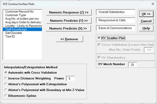
Available interpolation/extrapolation methods include:

Automatic with Cross Validation (default)
Inverse Distance Weighting with Power
Akima's Polynomial with Extrapolation
Akima's Polynomial with Boundary at Min Z Value (no extrapolation)
Biharmonic Spline.

The X and Y values may also be standardized which keeps both variables using the same units. An XY Scatterplot may be produced to view the coverage region (a.k.a. convex hull), beyond which extrapolation is required.

The choice of which interpolation/extrapolation method and settings are best to use is dependent on the data. Inverse Distance Weighting is more robust to outliers and sudden transitions than Akima or Biharmonic, but will not be as accurate for a smooth response.

Leave-One-Out Cross Validation may be used to assess the interpolation/extrapolation accuracy. Cross Validation R-Square and RMSE (root mean square error) are reported.If the maximum number of data points is exceeded (100 default), a random sample is used to keep the computation time reasonable.

The default Automatic with Cross Validation option will attempt Inverse Distance Weighting with Power values from 1 to 12, Akima's Polynomial with Extrapolation and Biharmonic Spline, each with and without XY Standardization. Leave-One-Out Cross Validation is used to measure the prediction accuracy and the method with lowest RMSE is selected.

For formula details and references, see the Appendix: XYZ Contour/Surface Plot.

XYZ Contour/Surface Plot - Example

Open Customer Data.xlsx. Click Sheet 1 Tab. Click SigmaXL > Graphical Tools >XYZ Contour/Surface Plot; if necessary, click Use Entire Data Table, click Next.

Select Overall Satisfaction, click Numeric Response (Z) >>; select Responsive to Calls, click Numeric Predictor(Y); select Ease of Communications, click Numeric Predictor (X). Check XY Scatter Plot. Use the default XY-Mesh Number = 20 and Interpolation/Extrapolation Method as Automatic with Cross Validation.

Click OK. The XYZ Contour and Surface Plots are produced:

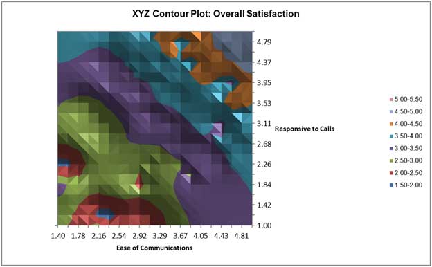
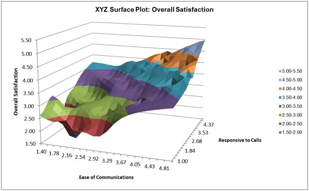
Clearly to maximize Overall Satisfaction, both Responsive to Calls and Ease of Communications must be maximized.

Tip: Excel's 3D Rotation Tool may be used by clicking on the chart, right-click and select 3D Rotation.

The Interpolation/Extrapolation and Cross-Validation report are given as:

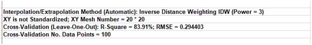
Inverse Distance Weighting with Power = 3 was selected by the Automatic Cross Validation method to produce the lowest RMSE. You can use Recall Last Dialog (or press F3) to experiment with other options.

The XY Scatter Plot is displayed as:

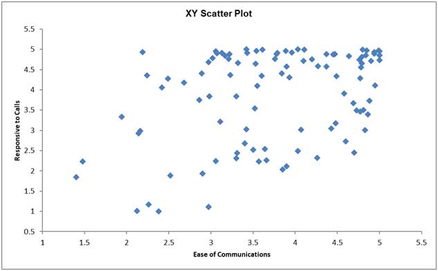
It is important to see where we do and do not have data coverage. High Ease of Communications with high Responsive to Calls are dense with data points so interpolation in this region will be more accurate. High Ease of Communications with low Responsive to Calls and High Responsive to Calls with low Ease of Communications have no data points so extrapolation is used and will be less accurate.