How Do I Create a One-Way ANOVA & Means Matrix in Excel Using SigmaXL?

One-Way ANOVA & Means Matrix

One-Way ANOVA and Means Matrix allows you to quickly do multiple pairwise comparisons. The One-Way ANOVA tests H0: μ1 = μ2 = μ3; Ha: at least one pairwise set of means are not equal.

Open Customer Data.xlsx, click on Sheet 1 tab.

Click SigmaXL > Statistical Tools > One-Way ANOVA & Means Matrix. Ensure that the entire data table is selected. If not, check Use Entire Data Table.
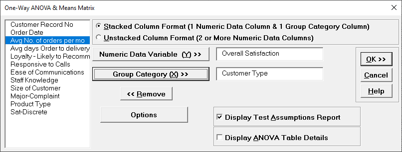
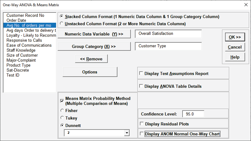
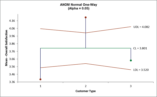
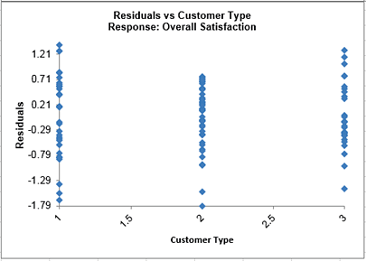
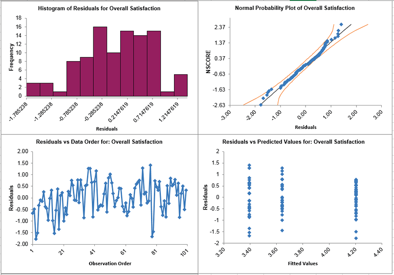
Click Next. Ensure that Stacked Column Format is checked. Select Overall Satisfaction, click Numeric Data Variable (Y) >>; select Customer Type, click Group Category (X) >>. Uncheck Display ANOVA Table Details.Check Display Test Assumptions Report.
Click OK. The results are shown below:

The ANOVA p-value of 0.0000 tells us that at least one pairwise set of means are not equal. From the Pairwise Mean Difference (Means Matrix), we conclude that Mean Overall Satisfaction is significantly different between Customer Type 2 and 3, as well as 1 and 2. Note that the default probabilities are Fisher Pairwise. The P-Values will be slightly different than the previous 2 Sample t-Test results because the variances from all 3 customer types are “pooled” here. This also results in slightly different confidence intervals. See below for more details on the multiple comparison options.

A graphical view of the Overall Satisfaction Mean and 95% Confidence Intervals are given to complement the Means Matrix. The fact that the CI’s for Customer Type 2 do not overlap those of Type 1 or 3, clearly shows that Customer Type 2 has a significantly higher mean satisfaction score. The overlap of CI’s for Type 1 and 3 shows that the mean satisfaction scores for 1 and 3 are not significantly different.

Note that the Confidence Level shown in the graph can be modified by clicking the Options button and setting Confidence Level. This also changes the alpha value used to highlight the PValues in red:

alpha = (100 – Confidence Level)/100

so the default Confidence Level = 95.0%, gives an alpha = 0.05
The R-Square (R-Sq) value of 20.95% indicates that Customer Type “explains” approximately 21% of the variation in Overall Satisfaction. We need to “drill down” to understand the root causes and best practices associated with Customer Type 2.
One-Way ANOVA Assumptions Report:

This is a text report with color highlight: Green (OK), Yellow (Warning) and Red (Serious Violation).

Each sample is tested for Normality using the Anderson Darling test. If not normal, the minimum sample size for robustness of the ANOVA Test is determined utilizing Monte Carlo regression equations (see Basic Statistical Templates – Minimum Sample Size for Robust t-Tests and ANOVA). If the sample size is inadequate, a warning is given and the appropriate Nonparametric test is recommended (Kruskal-Wallis if there are no extreme outliers, Mood’s Median if there are extreme outliers).

Each sample is tested for Outliers defined as: Potential: Tukey's Boxplot (> Q3 + 1.5*IQR or < Q1 – 1.5*IQR); Likely: Tukey's Boxplot 2*IQR; Extreme: Tukey's Boxplot 3*IQR. If outliers are present, a warning is given and recommendation to review the data with a Boxplot and Normal Probability Plot. Here we have a potential outlier for Customer Type 2.

Tip: If the removal of outlier(s) result in an Anderson Darling P-Value that is > 0.1, a notice is given that excluding the outlier(s), the sample data are inherently normal.

Each sample is tested for Randomness using the Exact Nonparametric Runs Test. If the sample data is not random, a warning is given and recommendation to review the data with a Run Chart.

A test for Equal Variances is also applied. If all sample data are normal, Bartlett’s Test is utilized, otherwise Levene’s Test is used. If the variances are unequal, then a warning is given and Welch’s ANOVA is recommended.

See Appendix Hypothesis Test Assumptions Report for further details.

One-Way ANOVA & Means Matrix - Options

Notes on Means Matrix Probability Method (Multiple Comparison of Means) and ANOM Chart:

Fisher:

Also known as Fisher’s Least Significant Difference (LSD)
Pairwise 2 sample t-tests with pooled standard deviation
Does not correct for family-wise error rate, so should only be used for k = 3 means and in the restricted case where the ANOVA P-Value is < alpha (this is also known as Protected Fisher LSD). For k = 3 means, Protected Fisher LSD is more powerful than Tukey.

Tukey:

Similar to LSD, uses pairwise tests with pooled standard deviation, but is a studentized range statistic that corrects for family-wise error rate. Recommended for k > 3.

Dunnett with Control:

If one of the groups are a control reference group, Dunnett with Control is more powerful than Tukey because it is doing fewer pairwise comparisons (only considers those pairwise against the control group).
Uses pooled standard deviation and a multivariate t distribution that corrects for family-wise error rate.

See Appendix Multiple Comparison of Means and Variances (a.k.a. Post-Hoc Tests) for further details and references.

Display ANOM Normal One-Way Chart:
- The ANOM alpha = (100 – Confidence Level)/100.
- This chart is also available at SigmaXL > Graphical Tools > Analysis of Means (ANOM). See Part P – Analysis of Means (ANOM) Charts.

Press F3 or click Recall SigmaXL Dialog to recall last dialog. Uncheck Display Test Assumptions Report. Click the Options button. Select Tukey. Check Display Residual Charts and Display ANOM Normal One-Way Chart; Confidence Level = 95.0 as shown:

Note: The Confidence Level is used to set the level in the Mean/Confidence Interval Plot, the alpha level (alpha = (100 – CI)/100) used to highlight the P-Values and the alpha level for the ANOM chart. However, the confidence level used in the Residuals Normal Probability Plot is always 95%.

Click OK. The Pairwise Means Difference (Means Matrix) and Tukey Probability results are:

The significant Tukey Probability values above have not changed as compared to Fisher, but note that they are larger than Fisher to compensate for the family-wise error rate:

Press F3 or click Recall SigmaXL Dialog to recall last dialog. Click Options. Uncheck all Display options and select Dunnett with Control Level = 2 (i.e. we are treating Customer Type 2 as the Control Group):

Click OK. The Pairwise Means Difference (Means Matrix) and Dunnett Probability results are:

All three mean differences are shown but only two probability values are calculated: Customer Type 1 – Control Type 2 and Control Type 2 – Type 3. (Typically, one would show 1 – 2 and 3 – 2 for Dunnett, but we are displaying the upper triangle for consistency with the other options).

Note that the Dunnett 2 – 3 P-Value is .003 which is smaller than the Tukey .004 but larger than the Fisher .002. Dunnett is more powerful than Tukey (due to having fewer tests), but less powerful than Fisher. It does, however, have an advantage over Fisher because it protects the family-wise error rate for the comparisons being made.

Click the ANOVA Residuals sheet tab to display the Residual Plots (created at steps 1, 2): Residuals

Residuals are the unexplained variation from the ANOVA model (Actual – Predicted/Fitted values). We expect to see the residuals approximately normally distributed with no obvious patterns in the above graphs, which is the case here.

Click ANOM_Normal_One_Way sheet tab to display the ANOM Chart (created at steps 1, 2):

Here we see that Customer Type 1 mean satisfaction score is significantly below the overall mean and Customer Type 2 is significantly higher. This is consistent with the results that are observed in the Pairwise Means Difference (Means Matrix), but is easier to interpret.

The varying decision limits are due to the varying sample sizes for each Customer Type, with smaller sample size giving wider limits in a manner similar to a control chart. If the data are balanced the decision limit lines will be constant.