Statistical Tools > General Linear Model > Fit General Linear Model
Extends Advanced Multiple Regression to include:
Fixed and Random Factors
Nested Factors
Covariates (can be Nested)
For Random or Mixed Random/Fixed Factors with a balanced design, the ANOVA and Variance
Components (VC) report is given based on Expected Mean Squares. VC confidence intervals
using Restricted Maximum Likelihood (REML) are included.
If the design is unbalanced or model is non-hierarchical, REML is used to compute the VC
values and confidence intervals. Fixed Effects Tests are based on Satterthwaite
approximation degrees of freedom.
Main Effects with Confidence Intervals and Interaction Plots of Fitted Means for
Non-Nested Fixed Factors
Tukey and Fisher Pairwise Comparison of Means for Non-Nested Fixed Factors
Predicted Response Calculator
Statistical Tools > General Linear Model > GLM Multiple Response Optimization
Multiple Response Optimization for Nested or Non-Nested Fixed Factors
Case study examples using GLM will be used to demonstrate the analysis of:
Fixed Factors with Nested Variable
Sources of Variation Study
Classical Gage R&R
Gage R&R Study with Operator as Fixed Factor
Destructive (Nested) Gage R&R
Expanded Gage R&R
Unbalanced Nested Factorial Experiment with Fixed and Random Factors
For further reading, the following book is recommended:
Montgomery, D.C. (2020). Design and Analysis of Experiments, 10th Edition, John Wiley &
Sons. See chapter 13 "Experiments with Random Factors" and chapter 14 "Nested and Split-Plot
Designs".
General Linear Model Dialogs and Options
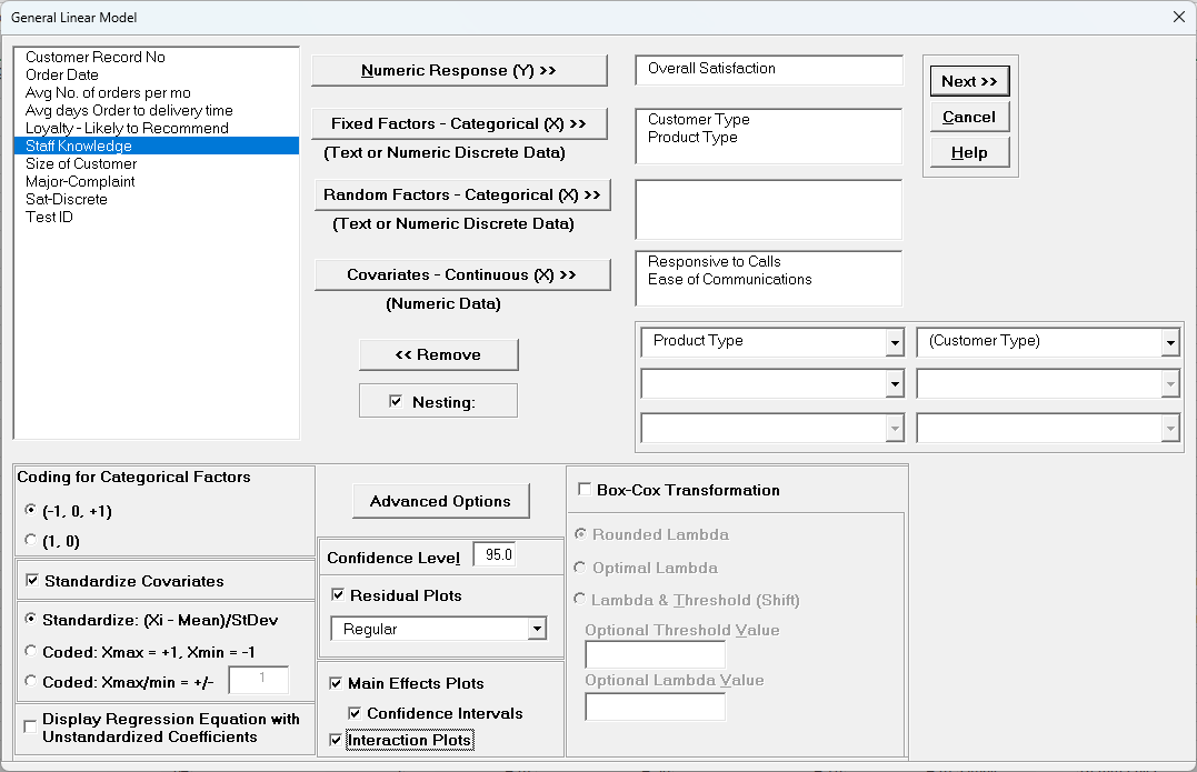
Fit General Linear Model Dialog
Numeric Response (Y) - select the response variable. Only one response
may be selected at a time, but you can use Recall SigmaXL Dialog or
Press
F3 to repeat an analysis with different options or to select a
different response. The regression reports will be created on sheetsGLM1 - Model
Y1name, GLM2 - Model Y2name, etc., but truncated
to fit the 31-character limit for Excel sheet names.
Fixed Factors - Categorical (X) - select fixed categorical predictors.
A fixed factor includes data for all levels of interest. Note, in previous analysis
using categorical predictors for One & Two-Way ANOVA and Multiple
Regression, the factors were assumed to be fixed.
Random Factors - Categorical (X) - select random categorical
predictors. A random factor has levels that are randomly sampled from a larger number of
possible levels but interest is in all possible levels. If a Random
Factor is selected, Advanced Options and Confidence
Intervals for Main Effects Plots are greyed out. A
variance components report will be produced in sheet GLM# - VarComp Yname.
Note that the GLM regression report treats random factors as fixed. ANOVA for
Predictors, Pareto Charts and CI/PI for Predicted Response Calculator are not available
in the regression report. See the variance components report for
analysis of random or random/fixed factors. Confidence Intervals for Main Effects Plots,
Stepwise/Best Subsets Regression, K-Fold Cross Validation, and Pairwise Comparison of
Means for Fixed Factors are not available.
For Fixed and Random Factors, numeric variables can be used but they will be converted
to text and an underscore "_" will be appended to the number. If there are more than 50
unique levels, a warning message is given. Typically, this
occurs when the user has incorrectly selected a continuous variable as categorical. Note
that the character "*" cannot be in the name as this is used to denote a cross product
term and will be error trapped. Parenthesis characters
"(" and ")" will be converted to underscore "_" since these are used to denote a nested
term.
Covariates - Continuous (X) - select continuous numeric variable of
interest. Selections with data as text are error trapped. Note that the character "*"
cannot be in the Covariate name as this is used to denote a
cross product term and will be error trapped. Parenthesis characters "(" and ")" will be
converted to underscore "_" since these are used to denote a nested term.
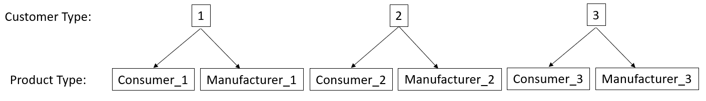
Nesting - check to include nested terms in the model. The left-side
combo dropdown selection can be a Factor or Covariate. The right-side dropdown selection
is a Factor. This will create a term with the notation A(B)
where A is nested in B. For the example above, that would produce Product Type(Customer
Type). The graphical representation of this is:
The product type "Consumer_1" is unique to Customer Type 1, etc.
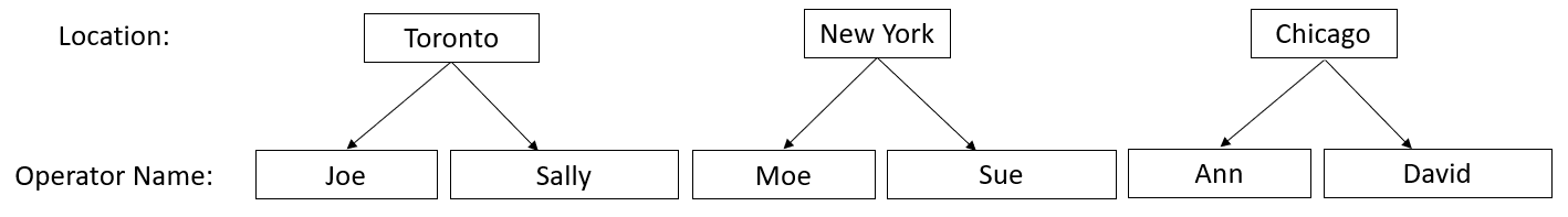
Another example
of a nested term would be Operator(Location) where the operators in each plant
location are different:
A
maximum of three levels of nesting are permitted with up to four factors. In the model,
this would appear as "D, C(D), B(C(D)), A(B(C(D)))" or "A, B(A), C(B(A)),
D(C(B(A)))" depending on the nesting assignment. One should exercise caution when using
three levels of nesting as the number of coefficients in the model is equal to the
number of factor combinations =
levelsA*levelsB*levelsC*levelsD.
A
factor cannot be nested within itself, either directly or indirectly, so model "A(B),
B(A)" or "A(B), B(C), C(A)" would be illegal.
Note,
"B(A), C(A)" is legal, but "A(B), A(C)" is illegal. A workaround to this limitation
would be to create a new factor "B_C" by concatenating the levels of B and C and using
"A(B_C)".
If B is nested in A, or A nested in B, i.e., B(A) or A(B), the interaction term
A*B is not permitted. SigmaXL automatically excludes these interactions in the Specify
Model Terms dialog. Interactions involving A or B with
other factors are permitted.
Term hierarchy in a model is recommended, but not
required.
Coding for Categorical Factors (-1, 0, +1), also known as effects
coding, estimates the difference between each factor level mean and the overall mean. It
results in lower multicollinearity VIF scores than (1, 0) coding. The
reference level is the last alpha-numerically sorted level and is hidden in the
Parameter Estimates table.
Coding for Categorical Factors (1, 0), also known as dummy coding, is
the coding scheme typically used for categorical predictors in a regression analysis.
The hidden reference value is the first alpha-numerically
sorted level.
Standardize Continuous Predictors with Standardize: (Xi -
Mean)/Stdev will convert continuous predictors to Z-scores. This has two
benefits: the predictors are scaled to the same units so coefficients can be
meaningfully compared, and it dramatically reduces the multicollinearity
VIF scores when interactions and/or quadratic terms are specified.
Standardize Continuous Predictors with Coded: Xmax = +1, Xmin =
-1 scales the continuous predictors so that Xmax is set to +1 and Xmin is
set to -1. This is particularly useful for analyzing data from a full or
fractional-factorial design of experiments.
Standardize Continuous Predictors with Coded: Xmax/Xmin = +/-
value scales the continuous predictors so that Xmax is set to +value
and Xmin is set to -value. This is particularly useful if one is analyzing data
from a response surface design of experiments, where
value is set to the alpha axial value such as 1.414 for a two-factor
rotatable design.
Display Regression Equation with Unstandardized Coefficients displays
the prediction equation with unstandardized/uncoded coefficients but the Parameter
Estimates table will still show the standardized coefficients.
This format is easier to interpret since there is only one coefficient value for each
predictor.
Confidence Level is used to determine what alpha value is used to
highlight P-Values in red, the significance reference line in the Pareto Chart of
Standardized Effects, and the percent confidence and prediction interval
used in the Predicted Response Calculator.
Residual Plots Regular display the raw residuals (Y - Ŷ) with a
Histogram, Normal Probability Plot, Residuals vs Data Order, Residuals vs Predicted
Values, Residuals vs Continuous Predictors and Residuals vs Categorical
Predictors.
Residual PlotsStandardized display the residuals, divided by
an estimate of its standard deviation. This makes it easier to detect outliers.
Standardized residuals greater than 3 and less than -3 are considered
large (these outliers are highlighted in red).
Residual PlotsStudentized (Deleted t)display studentized
deleted residuals which are computed in the same way that standardized residuals are,
except that the i
th observation is removed before performing the regression fit. This prevents
the ith observation from influencing the regression model, resulting in
unusual observations being more likely to stand out.
The Residuals report is provided on a separate sheet and includes a table with all
residual types to the left of the plots. Other diagnostic measures included, but not
plotted are Cook's Distance (Influence), Leverage and DFITS. Leverage
is a measure of how far an individual X predictor value deviates from its mean. High
leverage points can potentially have a strong effect on the estimate of regression
coefficients. Leverage values fall between 0 and 1. Cook's
distance and DFITS are overall measures of influence. An observation is said to be
influential if removing the observation substantially changes the estimate of model
coefficients. Cook's distance can be thought of as the product
of leverage and the standardized residual squared; DFITS as the product of leverage and
the studentized residual. These diagnostic measures can be manually plotted using a Run
Chart to identify unusually large values. Commonly
used rough cutoff criterion for Cook's distance are: > 0.5, potentially influential
and > 1, likely influential. A more accurate cutoff is the median of the F
distribution: > F(0.5,p,n-p), where n is the sample size and p is the
number of terms in the model design matrix, including the constant. A commonly used
cutoff criterion for the absolute value of DFITS
is:>2√(p/n)). An observation that is an outlier and
influential
should be examined for measurement error or possible assignable cause. You could also
try refitting the model excluding that observation to assess the influence.
The Residuals report also includes a table to the right of the plots with the stored
model design matrix and residuals. This can be used to manually create additional
residual plots such as residuals versus interaction or quadratic
terms.
Tip: For large datasets (> 1K) you may want to uncheck the
Residual
Plots in order to speed up the analysis.
Main Effects Plots with Confidence Intervals and
Interaction Plots use fitted means, not data means. If an interaction
term is not in the model, the interaction plot is still displayed, but it is shaded
grey. If the model is not hierarchical, these plots are not displayed.
Box-Cox Transformation with Rounded Lambda will solve
for an optimal lambda and is rounded to the nearest value of: -5, -4, -3, -2, -1, -0.5,
0, 0.5, 1, 2, 3, 4, 5. A 0 denotes a Ln(Y) transformation,
0.5 is the SQRT(Y), and 1 is untransformed. Threshold (Shift) is computed automatically
if the response data includes 0 or negative values, otherwise it is 0. Note that the
threshold is subtracted from the data so the value will
be negative in order to provide positive response values. Solving lambda is also
supported in Stepwise Regression. The reported Parameter Estimates, Model Summary,
Information Criteria, Validation, Test Statistics and Residuals
are for the Box-Cox transformed response. The Predicted Response Calculator
automatically applies an inverse transformation so that the predicted response,
confidence and prediction intervals are given in the original untransformed
units. Note, Lambda is solved to normalize the regression residuals, not the raw data.
It is solved using the classical Box-Cox formula but the actual transformation uses a
simple power transformation.
Box-Cox Transformation with Optimal Lambda uses the
range of -5 to +5 for Lambda. Threshold is computed automatically if the response data
includes 0 or negative values.
Box-Cox Transformation with Lambda &
Threshold(Shift) allows the user to specify Lambda and Threshold. Threshold
is typically 0, but if the response data includes 0 or negative values, a negative
threshold
value should be entered, such that when subtracted from the data, results in positive
response values.
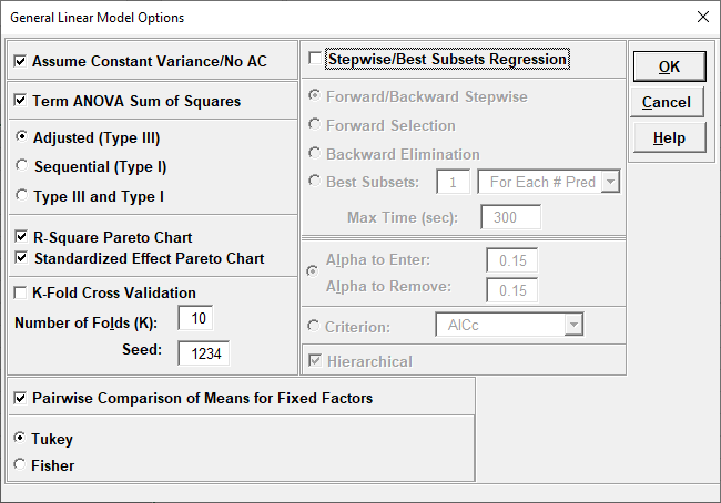
General Linear Model Options Dialog (not available if
Random Factor
selected)
Assume Constant Variance/No AC (no autocorrelation in the residuals),
if unchecked, SigmaXL will use either White robust standard errors for non-constant
variance or Newey-West robust standard errors for non-constant
variance with autocorrelation. If either of the Durbin-Watson P-Values are
< .05 (i.e., significant positive or negative autocorrelation), Newey-West for Lag 1
is used, otherwise White HC3 is used. This will affect SE Coefficients, P-Values, ANOVA
F and P-Values, and Prediction CI/PI. ANOVA F and P-Values are Wald estimates. ANOVA
SS Type I Table and Pareto Charts are not available. Note: Stepwise P-Values are not
adjusted.
Term ANOVA Sum of Squares with Adjusted (Type III)
provides a detailed ANOVA table for continuous and categorical predictors. Adjusted Type
III is the reduction in the error sum of squares (SS) when
the term is added to a model that contains all the remaining terms. Note, categorical
terms are considered as a group, unlike the parameter estimates table which uses
coding.
Term ANOVA Sum of Squares with Sequential (Type I)
provides a detailed ANOVA table for continuous and categorical predictors. Sequential
Type I is the reduction in the error sum of squares (SS) when
a term is added to a model that contains only the terms before it. This is affected by
the order that they are entered in the model, so the user must be careful to specify
model terms in the order of importance based on process
knowledge. Note, if the terms are orthogonal then Type III and Type I SS will be the
same.
R-Square Pareto Chart displays a Pareto chart of term R-Square values
(100*SS
term/SStotal). A separate Pareto Chart is produced for Type III
and Type I SS. If there is only one predictor term, a Pareto Chart is not
displayed.
Standardized Effect Pareto Chart displays a Pareto chart of term T
values (=T.INV(1-P/2,df
error)). A separate Pareto Chart is produced for Type III and Type I SS. A
significance reference line is included (=T.INV(1-alpha/2,dferror)).
K-Fold Cross Validation: In K-Fold cross-validation, the data is
randomly partitioned into K (approximately equal) subsets. The model coefficients are
estimated using K-1 partitions, i.e., (100*(K-1)/K)% of the data
- the training set, and then statistical metrics are evaluated on the remaining data -
the validation set. This is repeated for each of the K-Fold validation sets with
R-Square K-Fold and S (Standard Deviation) K-Fold calculated
as an average across the K samples, which results in a more accurate estimate of model
prediction performance. The default K=10 is a popular choice, but some practitioners
prefer K=5. Note that the final model parameter coefficients
are based on all of the data, so K-Fold Cross Validation is used strictly to obtain
R-Square K-Fold and S K-Fold. The fixed seed allows for replicable results, but the user
may wish to re-run the analysis with a different seed
a few times to see how much variation occurs in R-Square K-Fold and S K-Fold. If
categorical predictors are used and the training sample does not include all of the
levels, the K-Fold statistics cannot be computed.
Pairwise Comparison of Means for Fixed Factors: Tukey or
Fisher. Pairwise comparisons of means examines the difference between
all combinations of the estimated means for each category of a factor, along with the
standard error and confidence band for the difference.
Tukey provides protection against false positives due to multiple comparisons so is the
default selection. If the model is not hierarchical, the pairwise comparison report is
not available. For further information see the Appendix: Pairwise Comparison of Means for Fixed
Factors.
Stepwise/Best Subsets Regression with Forward/Backward
Stepwise: Starting with an empty model, terms are added or removed from the
model, one at a time, until all variables in the model have p-values that are less than
(or equal to) the specified Alpha-to-Remove and all variables that are
not in the model have p-values greater than the specified in
Alpha-to-Enter. The stepwise process either adds the term which is most
significant (largest F statistic, smallest p-value), or removes the term that is least
significant (smallest F statistic, largest p-value).
It does not consider all possible regression models. The independent variables can be
continuous and/or categorical. A categorical predictor is treated as a group, so is
either all in or all out.
Stepwise/Best Subsets Regression with Forward
Selection: Starting with an empty model, the most significant terms are
added to the model, one at a time, until all variables that are not in the model
have p-values greater than the specified in Alpha-to-Enter. Terms that
are in the model are not removed regardless of p-value. Alternatively, criterion-based
selection may be used. The most significant terms are
added, one at a time, while at each stage the value of a measure, such as AICc or
R-Square is monitored. If a minimum AICc is observed at step i, and this remains the
minimum after 10 additional steps (or the model includes all
terms), then the model at the minimum AICc is selected. If a maximum R-Square is
observed at step i, and this remains the maximum after 10 additional steps, then the
model with the maximum R-Square is selected. Criterion options
are: AICc, BIC, R-Square Adjusted, R-Square Predicted and R-Square K-Fold. AICc is the
Akaike Information Criterion corrected for small sample sizes, BIC is the Bayesian
Information Criterion. For details on these metrics, see
the Appendix: Advanced Multiple
Regression. Note that for R-Square K-Fold, the F-statistic to decide which term
to enter is based on all of the data. The K-Fold model is computed using the specified
model,
but a subset of the data is used as training data to estimate parameters and R-square is
calculated using the out-of-sample validation data. As with forward/backward stepwise,
the independent variables can be continuous and/or
categorical. A categorical predictor is treated as a group, so is either all in or all
out.
Stepwise/Best Subsets Regression with Backward
Elimination: Starting with all terms in the model, the least significant
terms are removed from the model, one at a time, until all variables in the model
have p-values that are less than (or equal to) the specified
Alpha-to-Remove. Terms that are removed from the model are not entered
again regardless of p-value. Alternatively, criterion-based selection may be used,
as described above, but the least significant terms are removed, one at a time. It stops
after 10 additional steps or if the model includes only one term. As with
forward/backward stepwise, the independent variables can be continuous
and/or categorical. A categorical predictor is treated as a group, so is either all in
or all out.
Stepwise/Best Subsets Regression with Best Subsets:
With Best Subsets, for any given model with p terms, there are 2p - 1
possible combinations (non-hierarchical models). A criterion such as AICc is
specified, and the model which results in the minimum AICc is selected. If p ≤ 15, all
possible combinations are explored - this is called exhaustive. Otherwise, the best
model is derived using discrete optimization with the powerful
MIDACO Solver (Mixed Integer Distributed Ant Colony Optimization). Start values are
obtained using forward selection with the AICc criterion. MIDACO does not guarantee a
best solution as we have in exhaustive, but will be close
to best, even for hundreds of terms! Best Subsets
Criterion options are: AICc, BIC and
R-Square Adjusted. R-Square Predicted and
R-Square K-Fold are not feasible as criterion here due to the computation
times, but
they are reported on the best selected models. Best Subsets report options are: Best
For Each # of Pred (default) or Best Overall. Best For Each # of
Predictors provides the most information but takes longer to compute than Best
Overall. The user may specify how many models to include (per # predictors or overall)
in the report, with the default = 1. The default Max Time (sec) = 300
is the maximum total computation time allotted for either
option. The independent variables can be continuous and/or categorical. A categorical
predictor is treated as a group, so is either all in or all out.
Stepwise/Best Subsets Regression - Hierarchical: The Hierarchical
option constrains the model so that all lower order terms that comprise the higher order
terms are included in the model. This is checked by default.
In Forward/Backward Stepwise and Forward Selection, a hierarchical model is required at
each step, but extra terms can enter to maintain hierarchy. For Backward Elimination and L14 (which
Best Subsets, extra terms are not permitted.
Saturated Model Pseudo Standard Error (Lenth's PSE): For saturated
models with dferror = 0, Lenth's method is used to compute a pseudo standard
error. For each term, a
t ratio is computed by dividing the coefficient by
the PSE. Since the distribution of the t ratio is not analytic, the probability
is evaluated using Monte Carlo simulation. Student T P-Values are also available for
comparison purposes. Lenth's PSE in the SigmaXL DOE Templates and
DOE Analysis use Student T P-Values.
Tip: There are a lot of options here, giving the user flexibility for model
refinement, but this can also be overwhelming to someone starting out with these tools. We
recommend using the following settings for Stepwise/Best Subsets
Regression:
Forward Selection, Criterion:AICc,
BIC or R-Square Predicted,
Hierarchical checked. This is fast and will build a model that
minimizes
AICc, BIC or maximizes R-Square Predicted.
AICc or R-Square Predicted are recommended for the best model
prediction accuracy,
BIC is recommended
for model parsimony. Note, however, this does not consider all possible models.
Best Subsets, 1 For Each # of Pred, Max Time
(sec) = 300,
Criterion: AICc or BIC, Hierarchical
checked. This can be slow but gives a very useful report of the best model for each
number of predictors in the model.
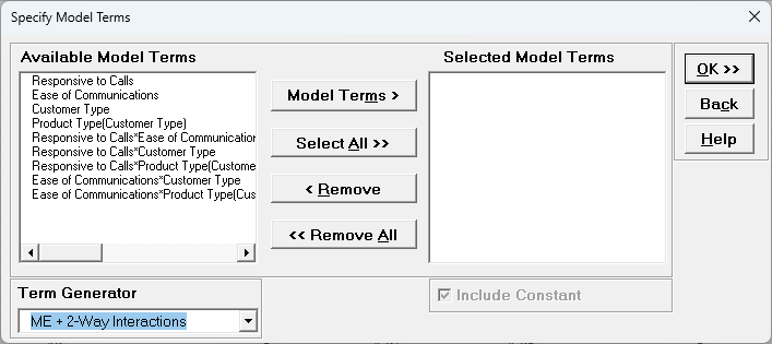
Specify Model Terms Dialog
Term Generator - select any of the following to build a list of
Available Model Terms:
Main Effects - default - no change to original specified terms
ME+ 2-Way Interactions - use this to include 2-way interactions in the
model, for example, analyzing data from a Res IV or Res V fractional-factorial DOE.
When specifying interactions or higher order terms, standardization
of continuous predictors is highly recommended.
ME + 2-Way Interactions + Quadratic - use this to include 2-way
interactions and quadratic terms in the model, for example, analyzing data from a
response surface DOE. Categorical terms will not be squared.
ME + All Interactions - use this to include all possible interaction terms
in the model, for example analyzing data from a full-factorial DOE.
All up to 3-Way - use this to include 2-way interactions, quadratic, 3-way
interactions, quadratic*main effect and cubic terms in the model. Categorical terms
will not be squared or cubed.
Model Terms: Select from highlighted Available Model
Terms.
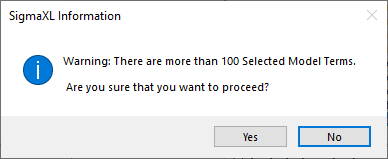
Select All: Select all Available Model Terms. Caution,
the number of selected terms can become quite large, especially for the last two options
in the
Term Generator. If more than 100 terms are selected, a warning is given
after clicking OK:
Include Constant: Always checked in GLM.
Tip: It is also important to ensure that the number of
rows/observations are sufficient to estimate the number of selected model terms. A rule
of thumb (excluding data from a designed experiment) is that for every
term selected, there should be a minimum of 10 rows of data. This rule holds for
potential terms used in stepwise and best subsets as well, otherwise one can easily
produce a model that is highly significant but a meaningless model
of noise. This is what Jim Frost calls “Data Dredging” in
chapter 8 of his book
Regression Analysis: An Intuitive Guide for Using and Interpreting Linear
Models.
Example 1: Fixed Factors with Nested Variable
Open Customer Data.xlsx. Click Sheet 1 Tab. Click
SigmaXL > Statistical Tools > General Linear Model > Fit General Linear
Model.
If necessary, click Use Entire Data Table, click
Next.
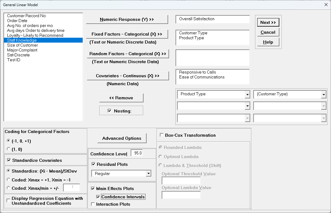
Select Overall Satisfaction, click Numeric Response (Y)
>>, select Customer Type and Product Type, click
Fixed Factors - Categorical (X) >>, select Responsive to
Calls and Ease of Communications, click Covariates -
Continuous (X) >>. Check Nesting.
For the left-side drop-down "Select a Factor or Covariate", select Product
Type.
For the right-side drop-down "Select a Factor to Nest in:" select (Customer
Type).
We will use the default Coding for Categorical Predictors (-1,0, +1).
Check Standardize Covariates with default option Standardize:
(Xi-Mean)/StDev.
Use the default Confidence Level = 95.0%. Regular Residual
Plots are checked by default.
Check Main Effects Plots with Confidence Intervals.
Leave Interaction Plots and Box-Cox Transformation
unchecked.
Tip: If you have covariates (continuous predictors) and are planning to
include interaction terms in the model, always ensure that Standardize
Covariates is checked. This has two benefits: the
covariates are scaled to the same units so coefficients can be meaningfully compared,
and it dramatically reduces the multicollinearity VIF scores.
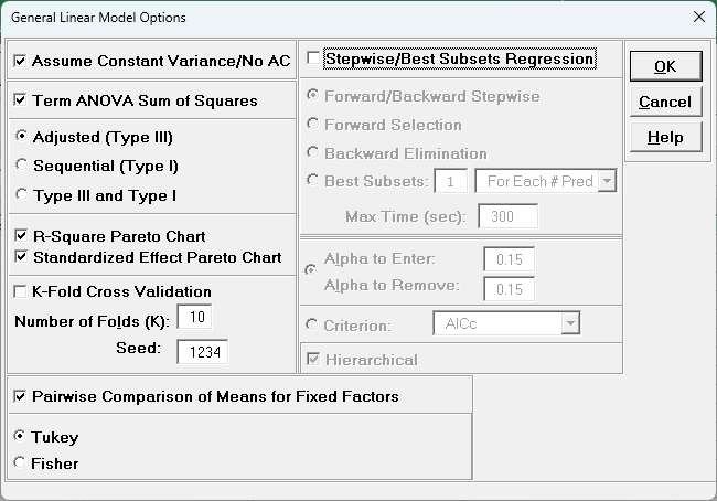
Click Advanced Options. We will use the default options as shown with
K-Fold Cross Validation and Stepwise/Best Subsets
Regression unchecked. Pairwise Comparison of Means for Fixed
Factors with
Tukey option is checked.
Click OK. Click Next >>.
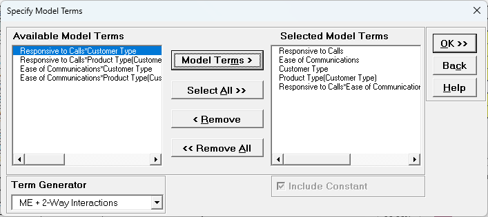
Using Term Generator, select ME + 2-Way Interactions. Select
Responsive to Calls to Responsive to Calls*Ease of Communication.
Click
Model Terms >. Include Constant is always checked in General Linear
Model.
Product Type(Customer Type) denotes that Product Type is nested within
Customer Type. Note, this data is not actually nested, but we are using this as
an example to demonstrate nesting with familiar data.
Term Generator, ME + 2-Way Interactions produces only legal
two-way interactions, so Product Type*Customer Type is not available for
selection. Based on previous regression analysis for Overall Satisfaction, we
are only including the Responsive to Calls*Ease of Communications 2-way
interaction.
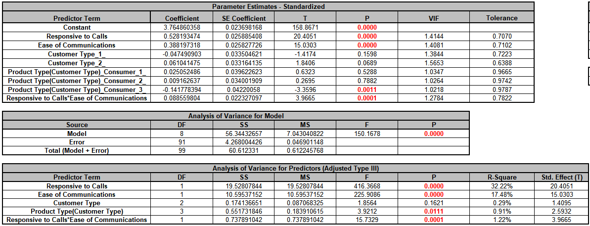
Click OK>>. The General Linear Model report is given. The
Parameter Estimates - Standardized and ANOVA tables are shown:
With (-1, 0, 1) coding, the reference level is the last alpha-numerically sorted level.
The hidden reference level for Customer Type is 3.
"Product Type(Customer
Type)_Consumer_1_" denotes Product Type Consumer nested within Customer Type 1. The
hidden reference level for Product Type is Manufacturer. For further information on
nesting see the Appendix: Nested Factors and
Coding.
The Analysis of Variance for
Predictors (Adjusted Type III) table shows that Customer Type is not
significant with P-Value = 0.162, but we will leave it in the model to maintain
hierarchy since Product Type is nested within Customer Type. Product
Type is significant with P-Value = 0.011.
The GLM Equation with standardized coefficients is:
General Linear Model: Overall Satisfaction = (3.76486)
Note blanks and special characters in the predictor names are converted to the
underscore character "_". The numeric Customer Type 1, 2, 3 has also been converted
to text so appear as "1_", "2_", "3_".
For categorical predictors, IF statements are used.
This is the display
version of the prediction equation given at cell L14 (which has more
precision for the coefficients and predictor names are converted
to legal Excel range names by padding with the underscore "_" character). If the
equation exceeds 8000 characters (Excel's legal limit for a formula is 8192), then a
truncated version is displayed and cell L14 does
not show the formula.
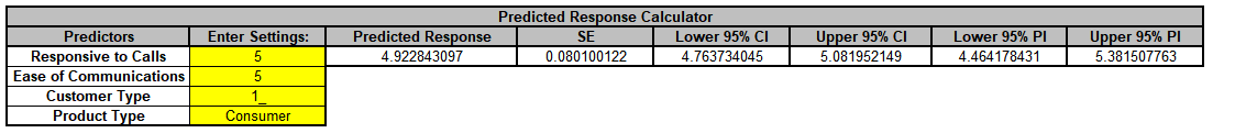
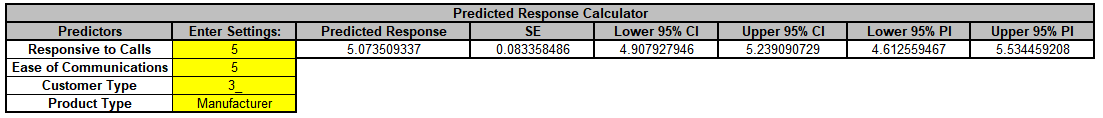
Scroll to the Predicted Response Calculator. Enter Responsive to Calls and
Ease of
Communication values = 5 with Customer Type = 1_ and Product Type = Consumer
from the dropdown lists to predict Overall Satisfaction including the 95% confidence
interval for the long term mean and 95% prediction interval
for individual values:
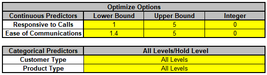
Next, we will use SigmaXL's built in Optimizer. Scroll to view the Optimize
Options:
Here we can constrain the continuous predictors and specify a level to use for
optimization of the categorical predictors. If a continuous predictor is integer,
change the Integer 0 to 1, and the Optimizer will return only integer
values for that predictor.
We will leave the Optimize Option settings as is.
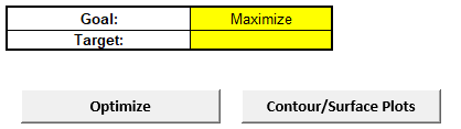
Scroll back to view the Goal setting and Optimize button. Select Goal =
Maximize.
The optimizer uses Multistart Nelder-Mead Simplex to
solve for the desired response goal with given constraints. For more information see the
Appendix: Single Response
Optimization.
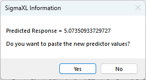
Click Optimize. The response solution and prompt to paste values into
the Input Settings of the Predicted Response Calculator is given:
Click Yes to paste the values.
The optimizer has selected Customer Type = 3_ and Product Type = Manufacturer to
maximize the Overall Satisfaction predicted value.
Note that the optimizer does not test the validity of a nested combination, so
if the goal is to optimize, it is best to use generic level names as done in this
example. For Product Type, we use the generic levels "Consumer"
and "Manufacturer", not "Consumer_Type1", "Consumer_Type2", "Consumer_Type3";
"Manufacturer_Type1", "Manufacturer_Type2", "Manufacturer_Type3".
Click on Sheet GLM1 - Pair Comp. The Tukey Pairwise Comparison of Means
for Customer Type is shown.
Pairwise comparisons of means examines the difference between all combinations of the
estimated means for each category of a factor, along with the standard
error and confidence band for the difference. Tukey provides protection against false
positives due to multiple comparisons. Nested factors are not shown in the pairwise
comparison report, so Product Type is not included here. For
further information see the Appendix: Pairwise
Comparison of Means for Fixed
Factors.
As expected from the ANOVA report, none of the pairwise
comparisons are significant.
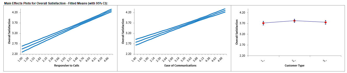
Click on Sheet GLM1 - Plots. The Main Effects Plots with 95%
Confidence Intervals are shown.
These are based on Fitted Means as predicted by the model, not Data Means. They use the
predicted value for the response versus input predictor value, while
holding all other variables constant. Continuous are held at their respective means and
categorical are weighted equally.
Here we see that Responsive to Calls has the steepest slope followed by
Ease of Communications. As expected, Customer Type does not appear to
be an important factor.
Example 2: Sources of Variation Study
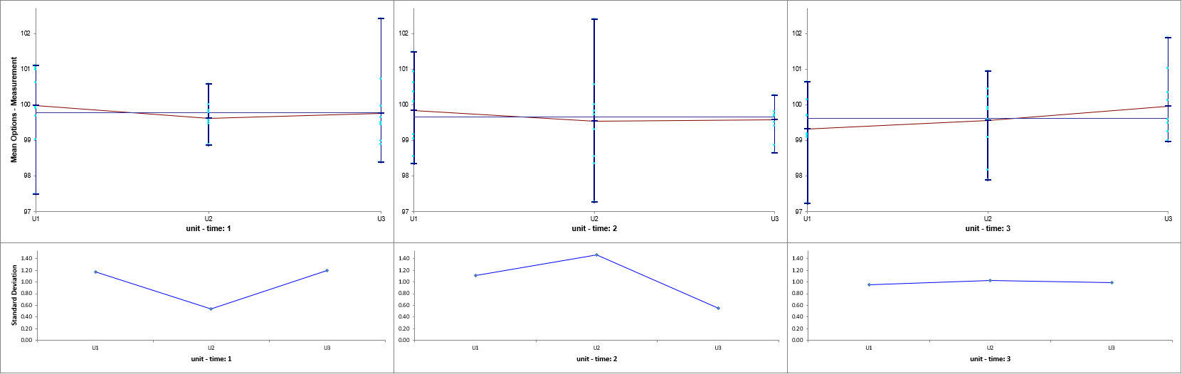
Open We will now reanalyze the Multi-Vari data presented in Multi-Vari Charts. The Multi-Vari chart was used to
identify dominant Sources of Variation (SOV), with the three major "families" of variation
being Within Unit, Between Unit, and Temporal (Over Time).
Dominant "Within Unit" Source of Variation:
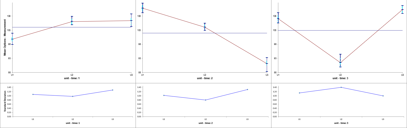
Dominant "Between Unit" Source of Variation:
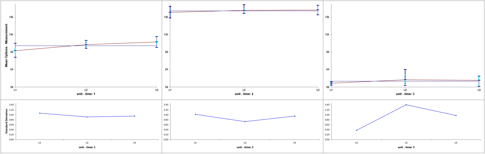
Dominant "Over Time" Source of Variation:
Unit and Time are Random Factors and Unit is nested within Time. The Variance Components
will be calculated to quantify the percent contribution to total variation for each
factor.
Open Multi-Vari Data.xlsx, click Sheet Within. Click
SigmaXL > Statistical Tools > General Linear Model > Fit General Linear
Model. If necessary, click Use Entire Data Table, click
Next.
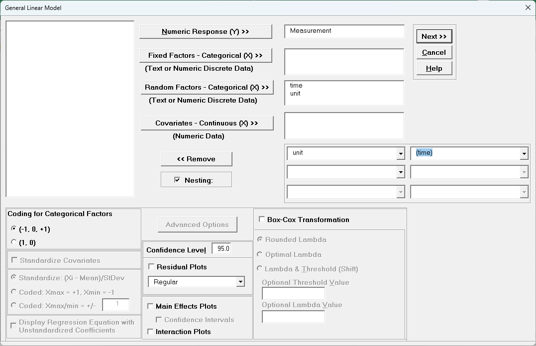
Select Measurement, click Numeric Response (Y) >>,
select
time, click Random Factors - Categorical (X) >>, select
unit, click Random Factors - Categorical (X) >>. Check
Nesting. For the left-side drop-down “Select a Factor or
Covariate”, select unit. For
the right-side drop-down “Select a Factor to Nest in:“, select
(time). We will use the default Coding for Categorical Predictors
(-1,0,
+1) and default Confidence Level = 95.0%. Leave
Residual
Plots, Main Effects Plots, Interaction Plots and Box-Cox
Transformation unchecked. Advanced Options are not
available with Random Factors.
Click Next >>.
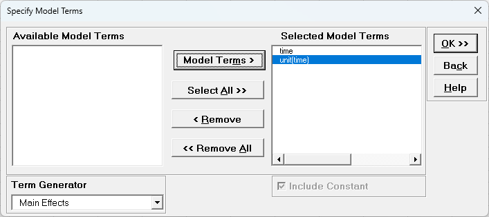
Leave Term Generator as Main Effects. Click Select All
>>. (If the order is reversed, select time, click Model Terms
>, select
unit(time), click Model Terms >.)
The term
unit(time) denotes that unit is nested within time. Since
time is the top level of the nesting, we place it in the model first.
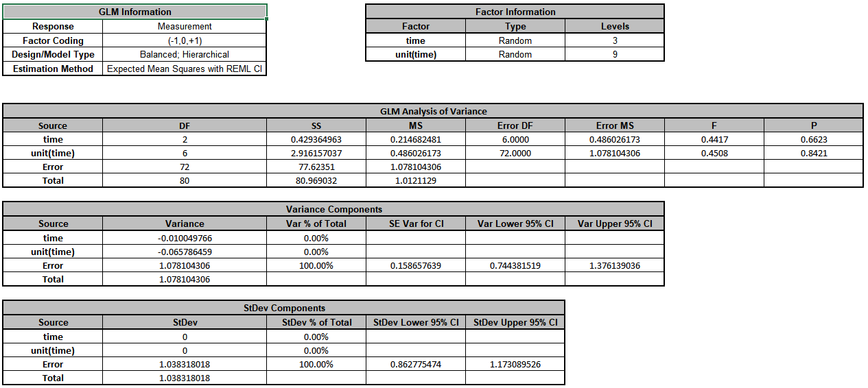
Click OK >>. The Variance Components report is given:
The
Error term in the variance components table is the “Within
Unit” variation. It is contributing to 100% of the total variation. The
REML 95% confidence interval for this variance component
is also given.
The terms time and unit(time) have negative Variance
Component values, so are treated as 0. The ANOVA table shows that both terms are not
significant random factors (alpha = 0.05). Standard Deviation
components are provided for convenience and useful in Measurement Systems Analysis, but
they will not be discussed here.
The GLM Model sheet is the regression analysis but we will not
review that here as our focus is on the variance components analysis. Note that the
regression analysis treats random factors as fixed.
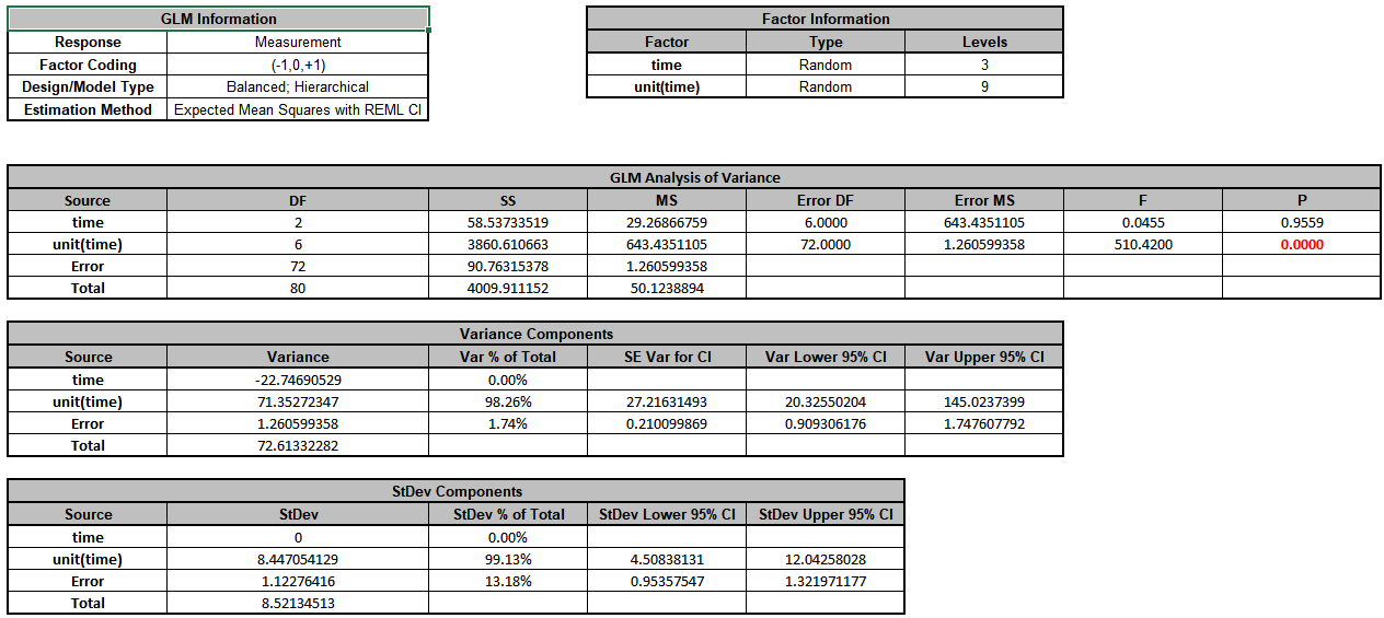
Now click sheet Between. Repeat steps 1 to 5 to produce the Variance
Components report:
The
unit(time) term in the variance components table is the “Between
Unit” variation. It is contributing to 98.3% of the total variation. The
“Within Unit”Error term is contributing to 1.7% of
the total variation. The REML 95% confidence interval for these variance components are
also given.
The term time has a negative Variance Component value, so is treated
as 0. The ANOVA table shows that time is not a significant random factor, but
unit(time) is significant (alpha = 0.05).
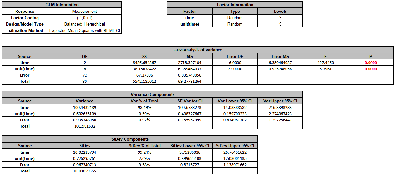
Now click sheet Over Time. Repeat steps 1 to 5 to produce the Variance
Components report:
The
time term in the variance components table is the “Over
Time” variation. It is contributing to 98.5% of the total variation. The
“Between Unit”unit(time) term is contributing to
0.6% of the total variation. The
“Within Unit” Error term is contributing to 0.9% of the total
variation. The REML 95% confidence interval for these variance components are also
given. Note that the confidence interval for time is very wide. This is due to
only having 3 levels. If possible, additional time value data should be collected in
order to reduce the uncertainty of the variance component value.
The ANOVA table shows that time and unit(time) are significant
random factors (alpha = 0.05).
Example 3: Classical Gage R&R Study
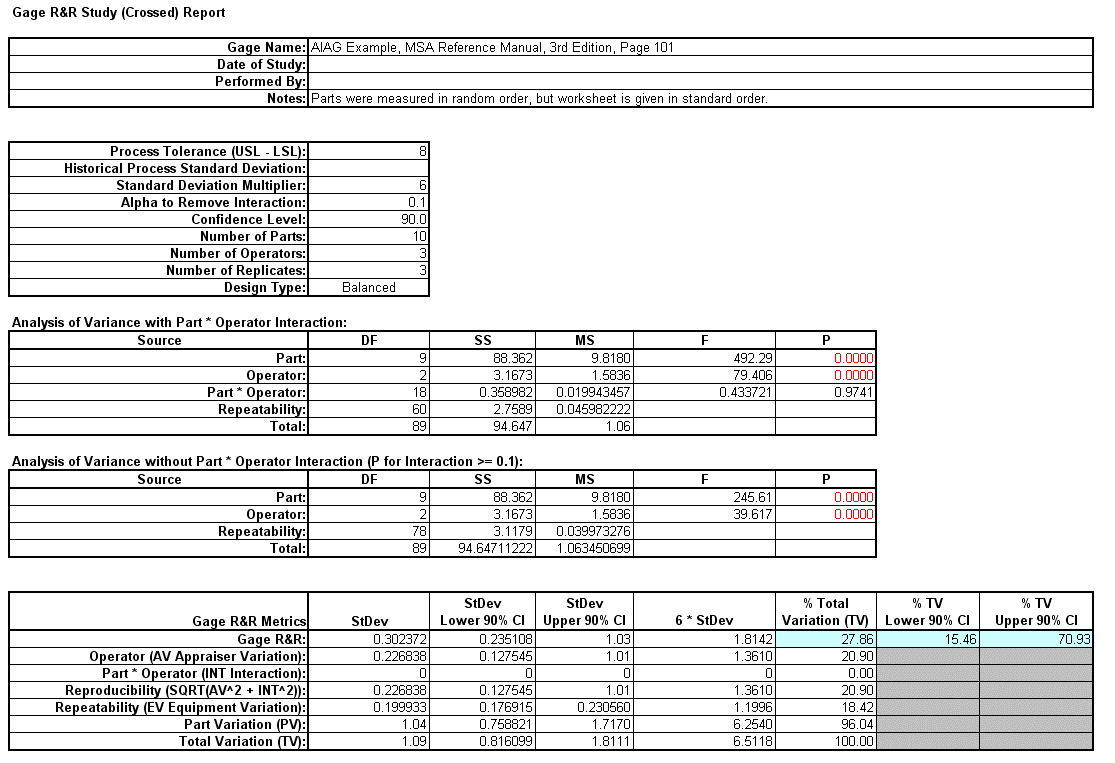
We will now reanalyze the AIAG Gage R&R data presented in Analyze Gage R&R (Crossed). The Gage R&R Study Report was given as:
Open the file Gage RR - AIAG.xlsx. This is an example from the Automotive Industry Action Group (AIAG) MSA Reference Manual, 3rd Edition, page 101. Note that parts were measured in random order, but the worksheet is
given in standard order. Preselect the worksheet data including column headings. Click
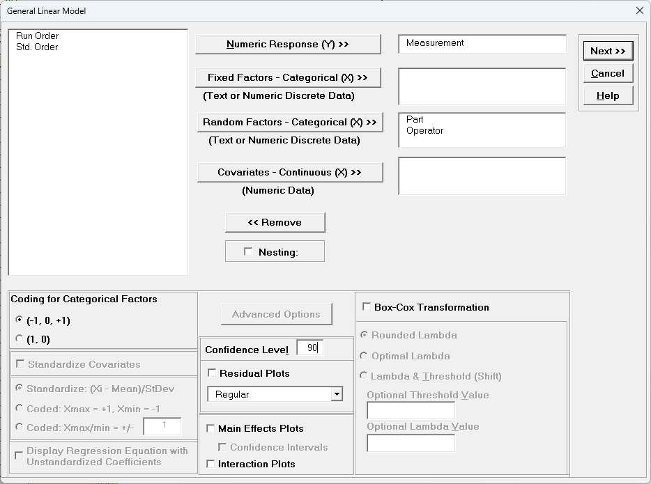
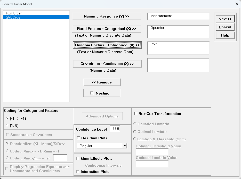
SigmaXL > Statistical Tools > General Linear Model > Fit General Linear Model. Click Next >>.
Select Measurement, click Numeric Response (Y) >>, select
Part and Operator, click Random Factors - Categorical (X) >>. Leave Nesting unchecked. We will use the default Coding for Categorical Predictors (-1,0, +1). Set
the
Confidence Level = 90% to match the previous Gage R&R analysis. Leave
Residual Plots, Main Effects Plots, Interaction Plots and Box-Cox
Transformation unchecked. Advanced Options are not available with Random Factors.
Click Next >>.
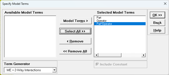
Using Term Generator, select ME + 2-Way Interactions. Click
Select ALL >>. Include Constant is always checked in General Linear Model.
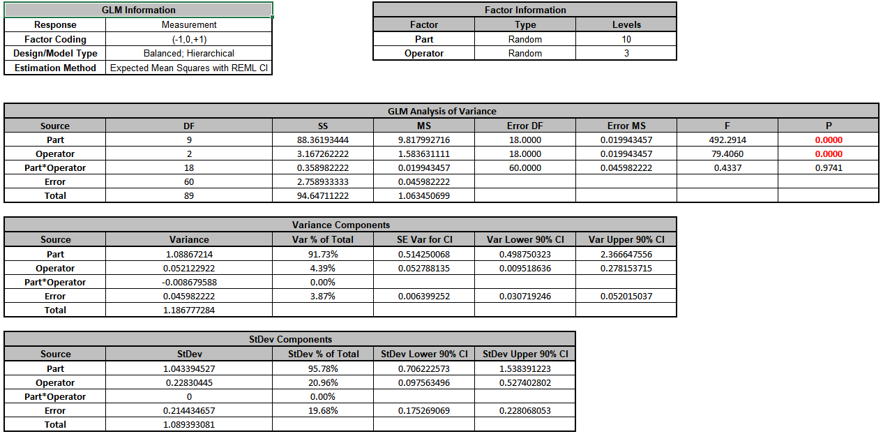
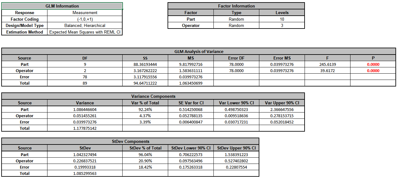
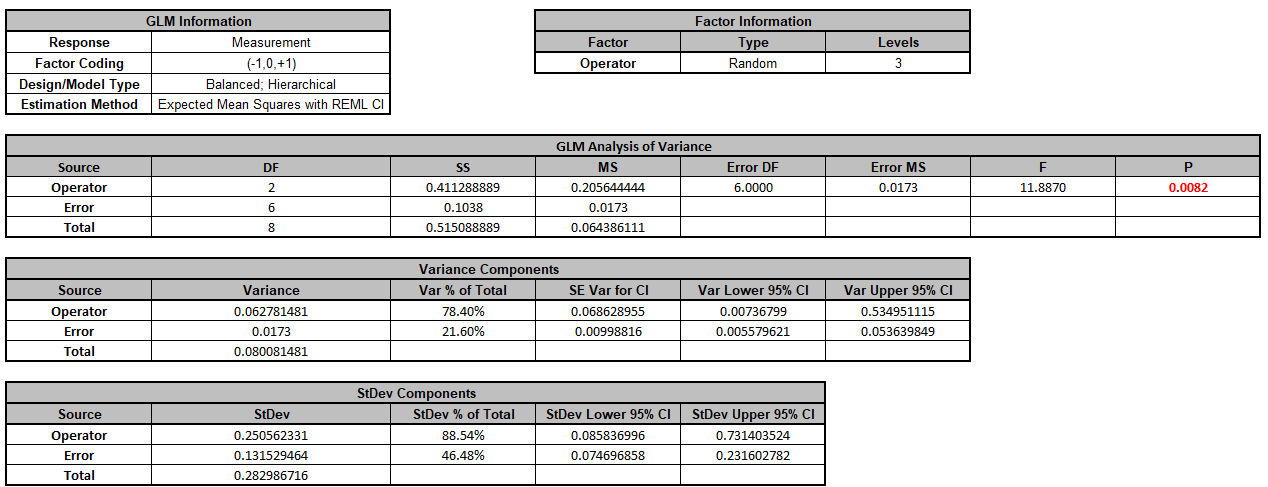
Click OK >>. The Variance Components report is given:
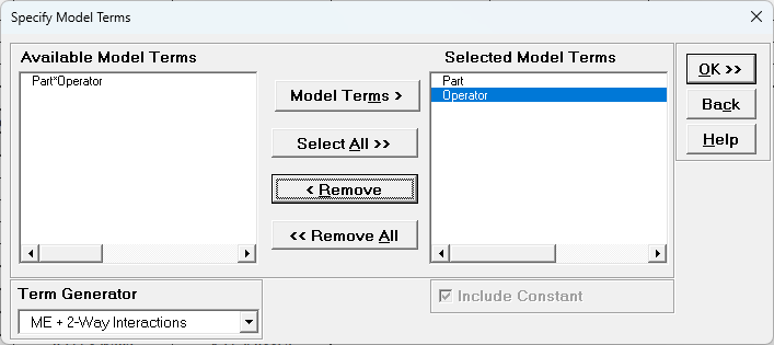
Since the Part*Operator interaction term is not significant (alpha = 0.1), we will refit the model excluding this term. Press F3 or click Recall SigmaXL
Dialog to Recall Last Dialog.
Click Next >>. Select Part*Operator,click
< Remove.
Click OK>>. The revised Variance Components report is shown:
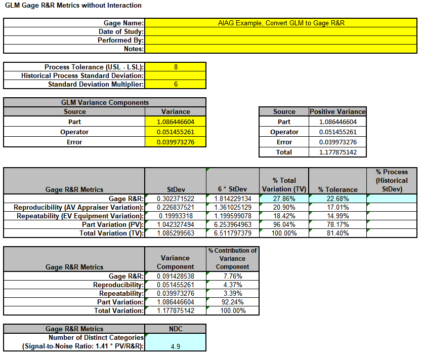
Now we will now convert the GLM Variance Components to Gage R&R Metrics. Click on
SigmaXL > Measurement Systems Analysis > Basic MSA Templates > GLM GageRR (Crossed)
Metrics without Interaction to open the conversion template.
Copy the Variance Component values in cells C18:C20 (Sheet GLM2
VarComp) and paste the values into the yellow highlighted cells
C15:C17 of the template. For Gage Name, enter the information as shown. Enter Process Tolerance =8, use Standard Deviation Multiplier = 6.
Warning: It is crucial to ensure that the GLM Variance Components Source Names match those given in the template. If the GLM model order was different than that of the template, each entry would have to be
copy/pasted individually.
This template converts the GLM Variance Components to Gage R&R metrics. The results match those given in the original analysis, excluding the confidence intervals and ANOVA table. With %Total Variation and %Tolerance less than 30%
but greater than 10%, this is a marginal measurement system.
Next, we will show examples where the classical Gage R&R Analysis does not work and GLM is required to do the analysis.
Example 4: Gage R&R Study with Operator as Fixed Factor
We will reanalyze the AIAG Gage R&R data above, but now we will treat Operator as a Fixed Factor. In this case “Operator” could denote a test fixture and there are only three of them in the plant.
Open the file Gage RR - AIAG.xlsx. Preselect the worksheet data including column headings. Click SigmaXL > Statistical Tools > General Linear Model > Fit General
Linear Model. Click Next>>.
Select Measurement, click Numeric Response (Y) >>, select
Operator, click Fixed Factors - Categorical (X) >>, select Part, click Random Factors - Categorical (X) >>. Leave Nesting unchecked. We will use the default Coding for Categorical Predictors (-1, 0, +1) and default
Confidence Level = 95.0%. Leave Residual Plots, Main Effects Plots,
Interaction Plots and Box-Cox Transformation unchecked.
Advanced Options are not available with Random Factors.
Click Next >>.
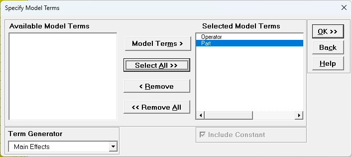
Leave Term Generator as Main Effects. Click Select ALL
>>.
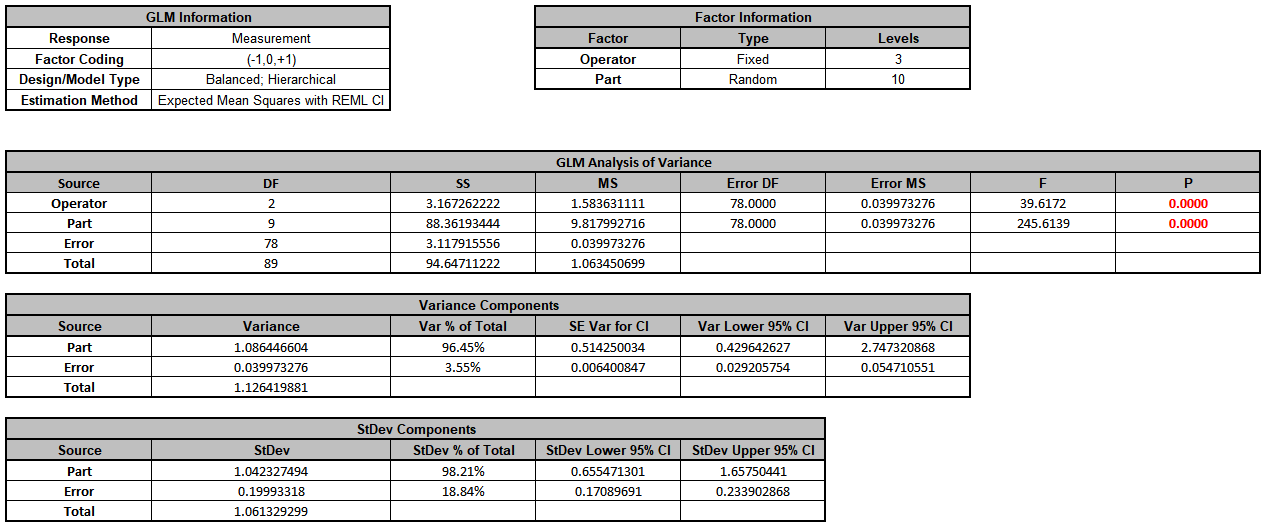
Click OK >>. The Variance Components report is given:
Note that Operator is no longer in the Variance Components table. We will need to manually calculate the VC value to be entered into the GLM GageRR template.
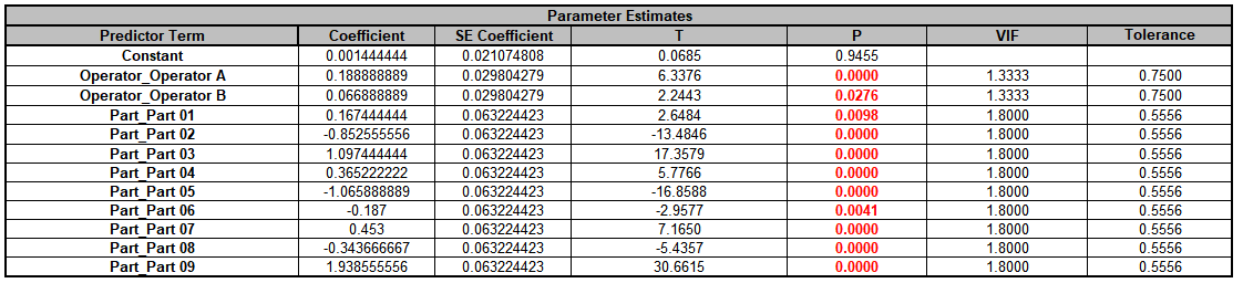
Click on Sheet GLM# Model for the current model. The Parameter Estimates are given as:
The coded (-1, 0, 1) coefficients for Operator will be used to estimate the Fixed Factor Variance Component. It is the average of the coefficients squared, including the hidden reference value. (This is from Formula
6.2 in Burdick, R. K., Borror, C. M., and Montgomery, D. C., “Design and Analysis of Gauge R&R Studies: Making Decisions with Confidence Intervals in Random and Mixed ANOVA Models”, ASA-SIAM
Series on Statistics and Applied Probability, 2005.) Note, this calculation cannot be done with coded (0, 1) coefficients.
Use Excel formulas to calculate this to full precision.
Now we will now convert the GLM and Manual Variance Components to Gage R&R Metrics. Click on
SigmaXL > Measurement Systems Analysis > Basic MSA Templates > GLM GageRR (Crossed)
Metrics without Interaction to open the conversion template.
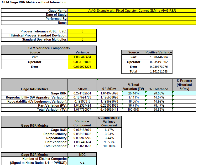
Enter the Variance Component values into the yellow highlighted cells C15:C17 of the template as shown. For Gage Name, enter the information as shown. Enter Process Tolerance =8, use Standard Deviation Multiplier
= 6.
Warning: It is crucial to ensure that the GLM Variance Components Source Names match those given in the template.
This template converts the GLM Variance Components to Gage R&R metrics. Note that the %Total Variation has been reduced from the original 27.86% to 25.44%, %Tolerance from 22.68% to 20.56% and NDC increased from 4.9 to 5.4. However, it is still considered
a marginal measurement system. Note that these steps should only be done when Operator is a fixed factor.
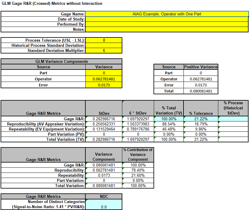
Example 5: Gage R&R Study with Operator and One Part
We will reanalyze the AIAG Gage R&R data, but now we will consider the case where there is only one part, i.e., like a Type 1 Gage R&R Study but with multiple operators.
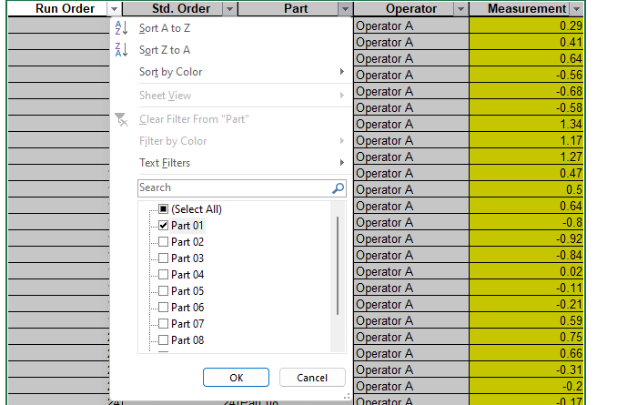
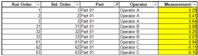
Open the file Gage RR AIAG.xlsx. Preselect the worksheet data including column headings. Click Excel > Data > Filter, select Part, uncheck Select All, check Part 01 as shown.
Click OK. This hides the rows for Parts 02 to 10.
Note: Three measurement readings per operator for a study with one part is not recommended. We are using this example with the AIAG data for convenience.
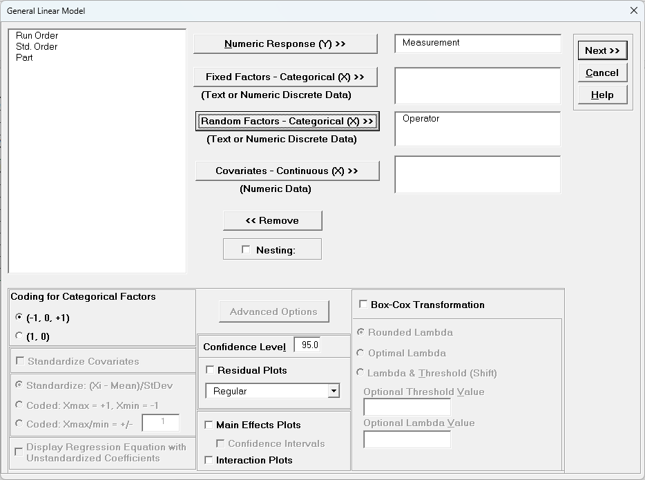
Click SigmaXL > Statistical Tools > General Linear Model > Fit General Linear Model. Click Next >>.
Select Measurement, click Numeric Response (Y) >>, select Operator, click Random Factors - Categorical (X) >>.
Leave Nesting unchecked.
We will use the default Coding for Categorical Predictors (-1, 0, +1) and default Confidence Level = 95.0%. Leave Residual Plots, Main Effects Plots, Interaction Plots and Box-Cox Transformation unchecked.
Advanced Options are not available with Random Factors.
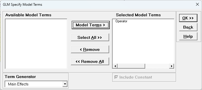
Click Next >>.
Click Model Terms >>.
Click OK >>. The Variance Components report is given:
Now we will now convert the GLM and Manual Variance Components to Gage R&R Metrics.
Click SigmaXL > Measurement Systems Analysis > Basic MSA Templates > GLM GageRR (Crossed) Metrics without Interaction to open the conversion template.
Copy the Variance Component values in cells C16:C17 (Sheet GLM# VarComp) and paste the values into the yellow highlighted cells C16:C17 of the template.
Enter 0 for Part Variance.
For Gage Name, enter the information as shown. Enter Process Tolerance =8, use Standard Deviation Multiplier = 6.
Warning: It is crucial to ensure that the GLM Variance Components Source Names match those given in the template.
This template converts the GLM Variance Components to Gage R&R metrics.
The %Total Variation is not applicable here because there is no part variation.
With %Tolerance less than 30% but greater than 10%, this is a marginal measurement system.
Example 6: Destructive (Nested) Gage R&R
We will now analyze data from a Destructive (Nested) Gage R&R found in the paper referenced below with link to the PDF. This is a shear test for a resistance spot welding process. Design of Experiments were used to produce the parts by varying preheat temperature, preheat current, welding temperature and welding current. Each run of a 4 Factor 8-Run Fractional Factorial DOE is a “Part” and this was replicated 6 times for a total of 48 welds. Two Shear Test machines were used so each machine tested 8 Parts with 3 Replicates. The shear test machines are the “Operator” and treated as a random factor in the study. Tensile Shear Strength (TSS Newtons) and Ultimate Strain (US mm) were measured, but we will only consider TSS here.
Open the file Tensile Shear Strength.xlsx. Click SigmaXL > Statistical
Tools > General Linear Model > Fit General Linear Model. If necessary, click
Use Entire Data Table, click
Next.
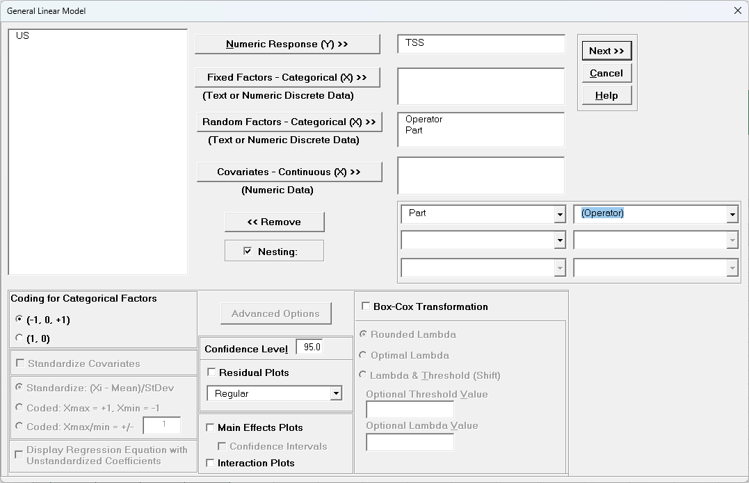
Select TSS, click Numeric Response (Y) >>, select Operator, click
Random Factors - Categorical (X) >>, select Part, click Random
Factors - Categorical (X) >>. Check
Nesting. For the left-side drop-down “Select a Factor or Covariate”, select
Part. For the right-side drop-down “Select a Factor to Nest in:”, select
(Operator). We will use the default Coding for Categorical Predictors (-1, 0,
+1) and default Confidence Level = 95.0%. Leave Plots,
Main Effects Plots, Interaction Plots and Box-Cox Transformation unchecked. Advanced Options are not available with Random Factors.
Click Next >>.
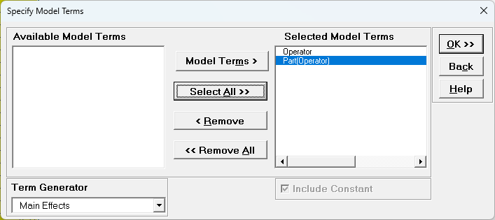
Leave Term Generator as Main Effects. Click Select ALL
>>.
The term Part(Operator) denotes that Part is nested within
Operator. Since Operator is the top level of the nesting, we place it in the model first.
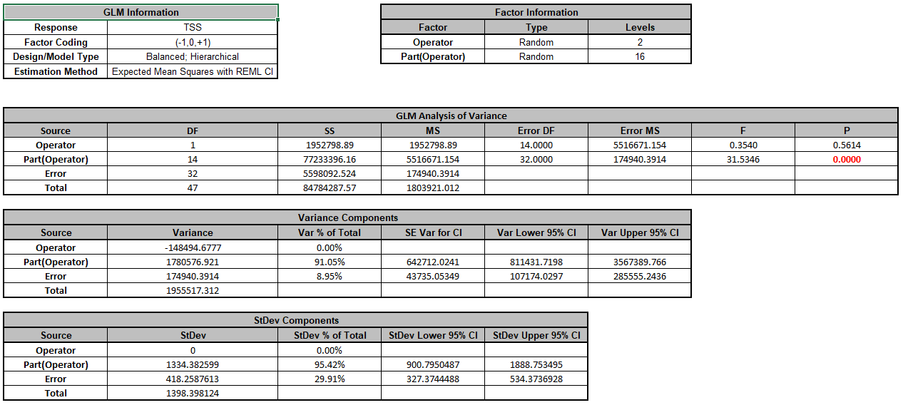
Click OK >>. The Variance Components report is given:
Note that Operator is a negative variance component. It will be treated as zero.
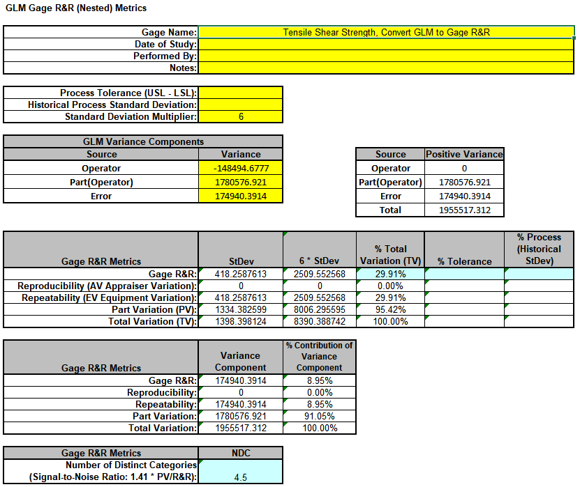
Now we will now convert the GLM Variance Components to Gage R&R Metrics. Click on
SigmaXL > Measurement Systems Analysis > Basic MSA Templates > GLM GageRR (Nested)
Metrics to open the conversion template.
Copy the Variance Component values in cells C18:C20 (Sheet GLM1 -
VarComp) and paste the values into the yellow highlighted cells C15:C17
of the template. For Gage Name, enter the information as shown. Use Standard Deviation Multiplier = 6.
Warning: It is crucial to ensure that the GLM Variance Components Source Names match those given in the template. If the GLM model order was different than that of the template, each entry would have to be copy/pasted
individually.
This template converts the GLM Variance Components to Gage R&R metrics. With %Total Variation less than 30% but greater than 10%, this is a marginal measurement system. The results match those given in the paper.
Example 7: Expanded Gage R&R
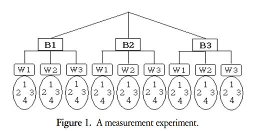
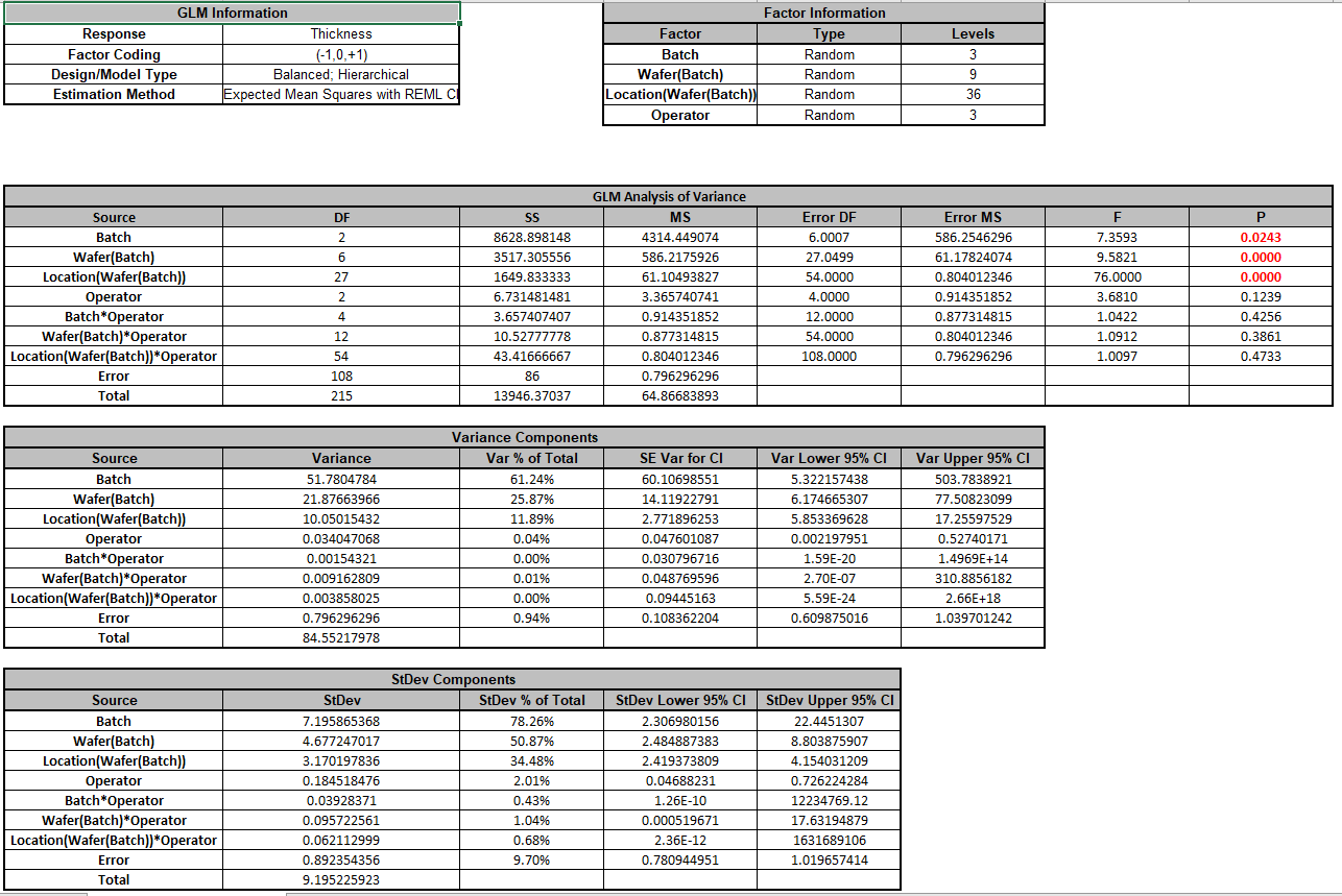
We will now analyze data from an Expanded Gage R&R found in the paper referenced below with link to the PDF. This is a wafer thickness measurement (Angstroms) for a semiconductor process. The design includes random factors: Batch, Wafer, Location and Operator. Wafer is nested within Batch and Location is nested within Wafer. There are 3 Batches, 3 Wafers, 4 Locations, 3 Operators and 2 Replicates for a total of 216 thickness measurements. The variance components for Part/Process include Batch, Wafer(Batch) and Location(Wafer(Batch)). The variance components for Reproducibility include Operator, Batch*Operator, Wafer(Batch)*Operator and Location(Wafer(Batch))*Operator. The variance component for Repeatability is the Error term from Replicates.
Reference: Lee, S.H., Lee, C.W. (2005), “A Study of Gage R&R Analysis Considering the Variations of Between-Within Group and Within Part”IE Interfaces 18(4), 444-453. https://koreascience.kr/article/JAKO200529256810322.pdf. Written in Korean but abstract, formulas, figures and tables are in English.
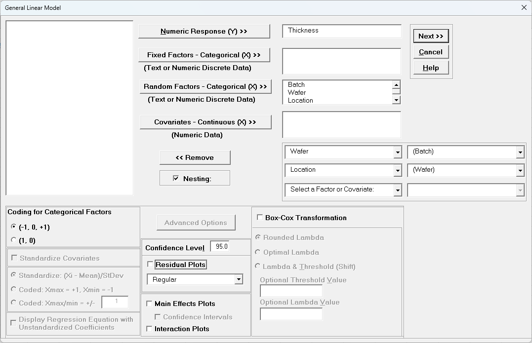
Open the file Wafer Thickness.xlsx. Click SigmaXL > Statistical Tools
> General Linear Model > Fit General Linear Model. If necessary, click Use
Entire Data Table, click Next.
Select Thickness, click Numeric Response (Y) >>, select Batch to
Operator, click Random Factors - Categorical (X) >>. Check
Nesting. For the left-side drop-down “Select a Factor or Covariate”, select Wafer. For the right-side drop-down “Select a Factor to Nest in:”,
select (Batch). For the second left-side drop-down “Select a Factor or Covariate”, select Location. For the right-side drop-down “Select a Factor to Nest in:”,
select (Wafer). We will use the default Coding for Categorical
Predictors (-1, 0, +1) and default Confidence Level = 95.0%. Leave Residual Plots, Main Effects Plots, Interaction Plots and
Box-Cox Transformation unchecked. Advanced Options are not available with Random Factors.
Click Next >>.
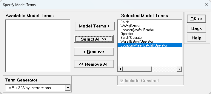
Using Term Generator, select ME + 2-Way Interactions. Click Select ALL >>.
The term Wafer(Batch) denotes that Wafer is nested within Batch. The term Location(Wafer(Batch)) denotes that Location is nested within Wafer which is nested within Batch. Only legal 2-Way Interactions are available, so Wafer*Batch, Location*Wafer or Location*Batch are not available.
Click OK >>. The Variance Components report is given:
Note that the variance component confidence intervals for the interaction terms with Operator are very wide and the P-Values are insignificant (alpha = 0.05), so the model could be refit excluding these terms but we will not do
so here.
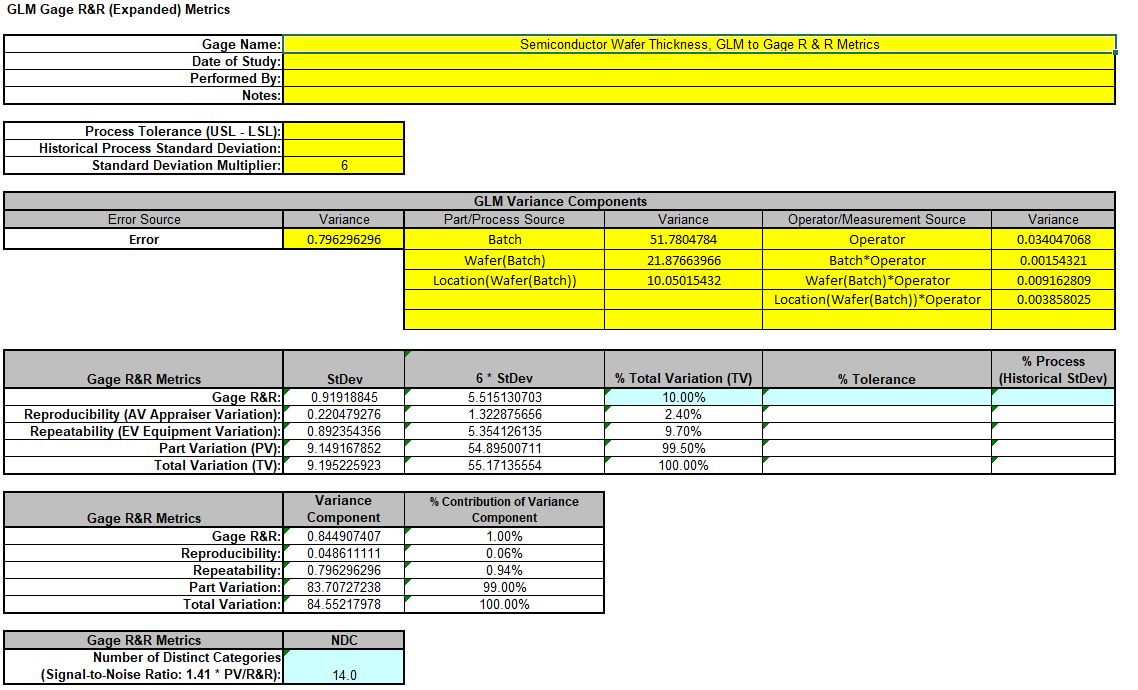
Now we will now convert the GLM Variance Components to Gage R&R Metrics. Click on SigmaXL > Measurement Systems Analysis > Basic MSA Templates > GLM GageRR (Expanded) Metrics to open the conversion template.
Copy the Variance Component values in Sheet GLM1 - VarComp and paste the values into the yellow highlighted cells of the template as shown. For Gage Name, enter the information as shown. Use Standard Deviation Multiplier = 6.
This template converts the GLM Variance Components to Gage R&R metrics. With %Total Variation = 10%, this is an acceptable measurement system. The results match those given in the paper.
Example 8: Analysis of a Split-Plot Experiment
Introduction to Split-Plot Designs
This introduction and example are based on two Quality Progress articles by Kevin J. Potcner and Scott M. Kowalski: “How to Recognize a Split-Plot Experiment” (Quality Progress, Nov 2003) and “How To Analyze A Split-Plot Experiment” (Quality Progress, Dec 2004).
While completely randomized designs are the standard for many experiments, they are not always efficient or realistic in industrial settings due to limitations in time, material, or equipment. A Split-Plot Design is often the solution when one or more factors are difficult or costly to change (Hard-to-Change), while others can be changed easily (Easy-to-Change).
Split-plot experiments originated in agriculture, where a "Whole Plot Factor" (like an irrigation method) was applied to a large section of land (the Whole Plot), and a "Subplot Factor" (like seed variety) was applied to smaller sections within that land (the Subplot).
Split-plot designs have three main characteristics that distinguish them from completely randomized designs:
Restricted Randomization: The treatment combinations are not assigned completely at random. The hard-to-change factor levels are fixed for a group of runs rather than being reset for every single run.
Different Experimental Units: The size of the experimental unit differs between factors. The Whole Plot factor is applied to a larger unit or group, while the Subplot factor is applied to individual units within that group.
Two Error Structures: Because of the two separate randomizations (Whole Plot and Subplot), the analysis must account for two different error variances: Whole Plot Error and Subplot Error.
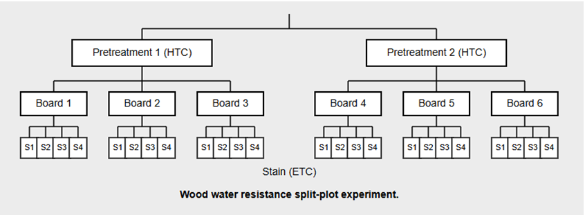
Experiment Background: Wood Resistance
This example utilizes the wood resistance experiment described in the Quality Progress articles. The objective is to study the effect of two factors on the water resistance of wood:
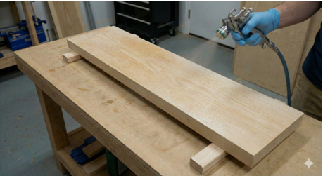
A single large wooden board is treated with one of the two types of pretreatment. This large board represents the Whole Plot.
In this experiment, the Pretreatment is the “hard-to-change” factor. Because it's difficult to apply the pretreatment to many small, individual pieces of wood, a single type of pretreatment is applied to an entire large board at once. This large board is the Whole Plot.
Applying Pretreatment to the Whole Plot.
Step 2: Creating the Subplots
Once the pretreatment has been applied to the whole board, it is cut into four smaller panels. These smaller pieces are the Subplots.
Step 3: The Subplot (Easy-to-Change Factor)
The “easy-to-change” factor, Stain, is applied to each of the smaller pieces. Since it is easy to change the stain from one piece to the next, each of the four pieces cut from the same original board can receive a different stain type in different random order.
Applying Stains to the Subplots.
This sequence of operations defines the split-plot structure, where the randomization of the pretreatment is restricted to the whole board, while the randomization of the stain is applied freely to the smaller pieces within that board.
Design Structure
Whole-Plot Factor (Hard to Change): Pretreatment (2 Levels, 3 Replicates per level = 6 Boards).
Sub-Plot Factor (Easy to Change): Stain (4 Levels).
Random Factor: Whole Plot (The 6 Boards).
Total Observations: 6 Boards x 4 Stains = 24 Runs.
In this analysis, we define Board, the Whole Plot, as a random factor nested within Pretreatment. This structures the model to estimate the Whole Plot error separate from the Subplot error.
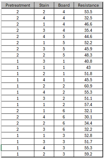
We will begin with a graphical view of the data using a Variability Chart. Open the file Wood Resistance Split Plot.xlsx.
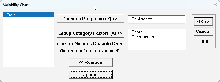
Click SigmaXL > Graphical Tools > Variability Chart. If necessary, click Use Entire Data Table, click Next.
Select Resistance, click Numeric Response (Y) >>. Select Board, click Group Category Factors (X) >>; Select Pretreatment, click Group Category Factors (X) >> as shown:
The innermost group is specified first. In this example it is Board which is the second lowest level on the tree diagram. The lowest level, Stain, will appear as a vertical line in the variability chart. We will use the default Options.
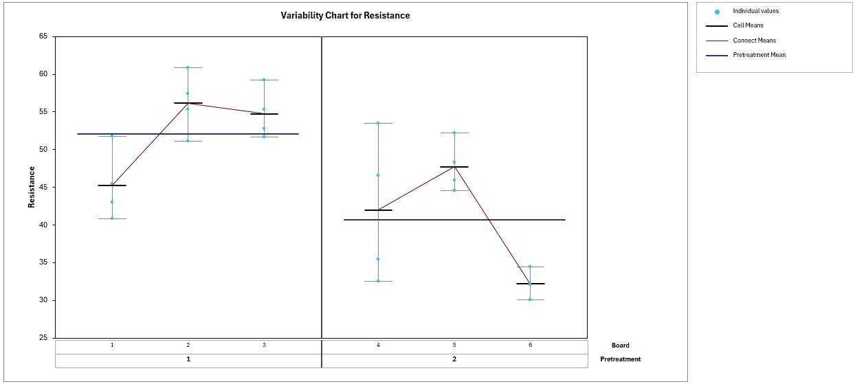
Click OK. The resulting Variability Chart is shown:
Several features of the data are immediately apparent. The blue horizontal lines show the Pretreatment means: Pretreatment 1 averages approximately 52 while Pretreatment 2 averages approximately 41. This looks like a large difference, but the board-to-board variation within each pretreatment level tells a different story. Within Pretreatment 1, the board means range from about 45 (Board 1) to 56 (Board 2). Within Pretreatment 2, the range is even wider — from about 32 (Board 6) to 48 (Board 5). This suggests that the apparent pretreatment difference may not be distinguishable from the natural variation between boards. In contrast, the within-board variation (the spread of individual values around each cell mean) is relatively small. This is encouraging for detecting Stain effects, since Stain differences are evaluated within boards where the noise is much smaller.
The Standard Deviation chart reinforces this observation: Most boards have a within-board standard deviation between 2 and 5, with Board 4 being a notable exception at nearly 10. This chart highlights that wood is a highly variable natural material, and the dominant source of variation appears to be between boards rather than within boards.
In summary, the Variability Chart foreshadows what the formal analysis will confirm: the large board-to-board variation (the whole plot error) will make it difficult to detect the Pretreatment effect, while the relatively small within-board variation (the subplot error) will provide good sensitivity for detecting Stain differences.
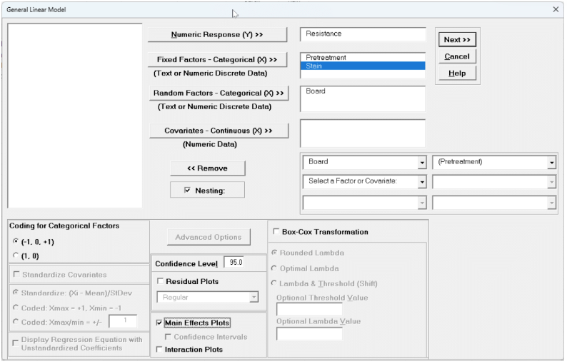
Click on the Sheet Variability Data. Click SigmaXL > Statistical Tools > General Linear Model > Fit General Linear Model. If necessary, click Use Entire Data Table, click Next.
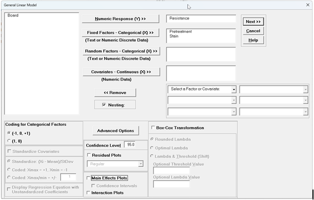
Select Resistance, click Numeric Response (Y) >>; select Pretreatment and Stain, click Fixed Factors - Categorical (X) >>; select Board, click Random Factors - Categorical (X) >>. Check Nesting. For the left-side drop-down "Select a Factor or Covariate", select Board. For the right-side drop-down "Select a Factor to Nest in:", select (Pretreatment). We will use the default Coding for Categorical Predictors (-1, 0, +1) and default Confidence Level = 95.0%. Check Main Effects Plots. LeaveInteraction Plots, Residual Plots and Box-Cox Transformation unchecked. Advanced Options are not available with Random Factors.
Click Next >>.
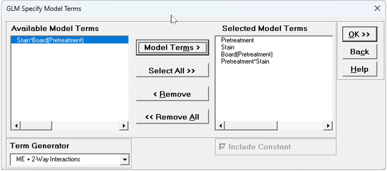
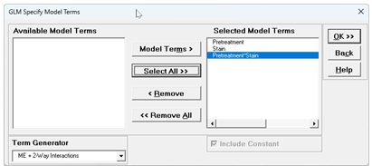
Using Term Generator, select ME + 2-Way Interactions. Select the Model Terms as shown:
The term Board(Pretreatment) denotes that Board is nested within Pretreatment. This random term serves as the error term for testing the Pretreatment effect. The Pretreatment*Stain interaction is included in the model. The Stain*Board(Pretreatment) interaction, the subplot error, is kept out of the model, otherwise there would be 0 degrees of freedom in the Error term.
Only legal 2-Way Interactions are available, so Board*Pretreatment is not available.
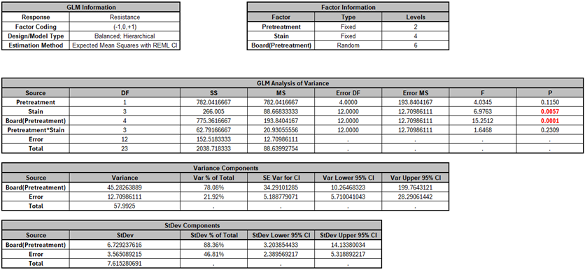
Click OK. The ANOVA and Variance Components report is given:
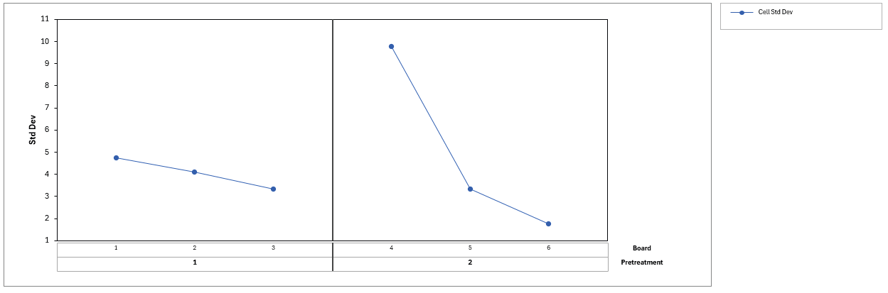
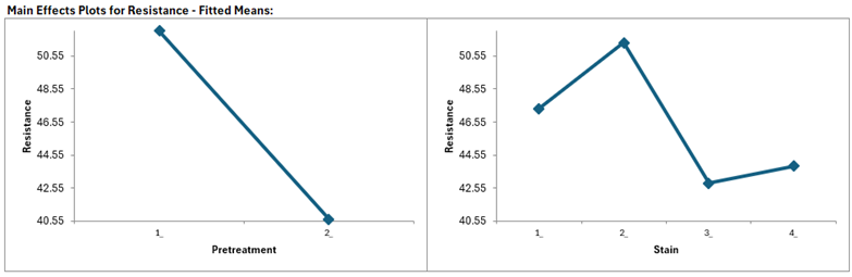
The Main Effects Plots are given as:
The Pretreatment factor is not statistically significant (P-Value = 0.115). Even though the Main Effects Plot shows a steep slope (dropping from 52.1 to 40.65), the analysis cannot prove this is a real effect.Pretreatment is tested against the Board(Pretreatment) error term which is very large (Mean Square = 193.84). Furthermore, the Variance Components table shows that Board(Pretreatment) = 78.1% of total variance in the experiment; this variation comes from the wood boards themselves. Because Pretreatment is the “Whole Plot” factor, it must overcome this huge noise to be declared significant.
The Stain factor is highly significant (P-Value = 0.006). This confirms that there is a real, detectable difference between the 4 stain types. Stain 2 is the best performer (highest resistance), while Stain 3 is the worst. Stain is tested against the Residual Error(Mean Square = 12.71), which is 15 times smaller than the board error. The Variance Components table shows that Error = 21.9% of total variance (i.e., within board). Because Stain is the "Subplot"� factor, it only has to overcome this small noise.
The fact that Board(Pretreatment) is significant (P-Value = 0.0001) confirms that the Boards are significantly different from each other (i.e., the wood is a highly variable natural material). The Split-Plot design has effectively blocked against this variation, allowing a more powerful evaluation of the Stain factor.
The Pretreatment*Stain interaction term is not significant (P-Value = 0.231): There is no evidence that the effect of the Stain depends on which Pretreatment was used. We could remove this term and refit the model but we will not do so here — the changes to the P-Values are negligible.
These results are in agreement with those given in the Potcner & Kowalski (2004) Quality Progress article.
Next, we will incorrectly re-analyze the data in this experiment, treating it not as a Split-Plot design but as a completely randomized design, as was done in the article.
Click Recall Last Dialog (or press F3).
Double-click on Board to remove it from the model (or select it and click << Remove). Uncheck Main Effects Plots.
Click Next >>. Using Term Generator, select ME + 2-Way Interactions. Select the Model Terms as shown:
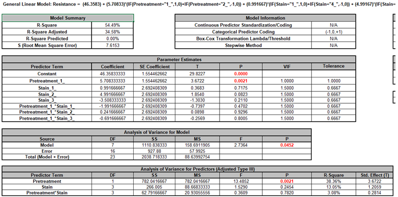
Click OK. The GLM Regression report is shown:
Looking at the Analysis of Variance for Predictors (Adjusted Type III) table, we see that Pretreatment is significant with P-Value = 0.002 and Stain is not significant with P-Value = 0.245. These are the reverse conclusions that were obtained from the correct Split-Plot analysis. This clearly demonstrates the importance of properly recognizing and analyzing a Split-Plot design.
References
Kowalski, S. M., & Potcner, K. J. (2003). "How To Recognize A Split-Plot Experiment". Quality Progress, 36(11), 60-66.
Potcner, K. J., & Kowalski, S. M. (2004). "How To Analyze A Split-Plot Experiment". Quality Progress, 37(12), 67-74.
Example 9: Unbalanced Nested Factorial Experiment with Fixed and Random Factors
We will now analyze a nested factorial experiment adapted from Example 14.2 in Montgomery's Design and Analysis of Experiments book. The process is the hand insertion of electronic components on printed circuit boards and the goal of the study is to improve the speed of the assembly operation. The design includes three assembly fixtures and two workplace layouts. Operators are required to perform the assembly.
In the book, four operators are randomly selected for each fixture-layout combination, but here we will use 4 operators for layout 1, but three for layout 2 making it an unbalanced design. The operators chosen for layout 1 are different individuals from those chosen for layout 2, so operators are nested within layout. Because there are only three fixtures and two layouts, these are fixed factors but the operators are random factors, so this is a mixed model. The treatment combinations in this design are run in random order, but the worksheet is shown in standard order. Two replicates are obtained. The assembly times are measured in seconds.
Since the design is unbalanced, SigmaXL will automatically use Restricted Maximum Likelihood (REML) to calculate variance components rather than the traditional ANOVA Expected Means Squares (EMS) method
Reference: Montgomery, D.C. (2020). Design and Analysis of Experiments, 10th Edition, John Wiley & Sons.
Open the file Assembly Time Nested Factorial.xlsx. Click SigmaXL > Statistical Tools > General Linear Model > Fit General Linear Model. If necessary, click
Use Entire Data Table, click Next.
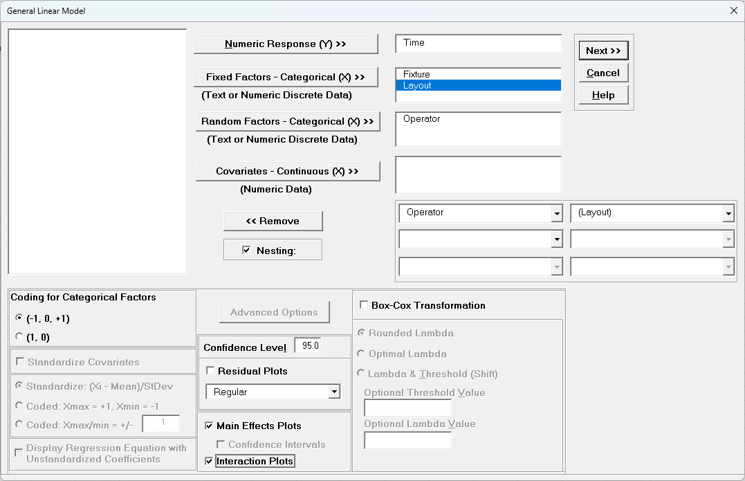
Select Time, click Numeric Response (Y) >>, select Fixture and Layout, click Fixed Factors - Categorical (X) >>, select Operator, click Random Factors - Categorical (X) >>. Check
Nesting. For the left-side drop-down “Select a Factor or Covariate”, select Operator. For the right-side drop-down “Select a Factor to Nest in:“,
select (Layout). We will use the default Coding for Categorical Predictors (-1, 0, +1) and default Confidence Level = 95.0%. Check Main Effects Plots and Interaction Plots. Leave
Residual Plots, and Box-Cox Transformation
unchecked. Advanced Options are not available with Random Factors.
Click Next >>.
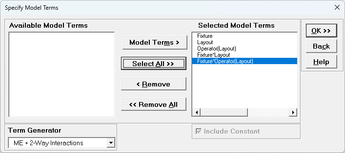
Using Term Generator, select ME + 2-Way Interactions. Click Select ALL >>.
The term Operator(Layout) denotes that Operator is nested within Layout. Only legal 2-Way Interactions are available, so Operator*Layout is not available.
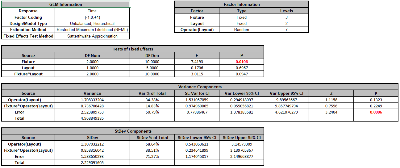
Click OK >>. The Variance Components report is given:
Since this is an unbalanced design, Restricted Maximum Likelihood (REML) is used to estimate the variance components. In Tests of Fixed Effects, we see that Fixture is significant but Layout and
Fixture*Layout are not significant. In Variance Components, Operator(Layout) contributes to 34.4% of the total variance and the interaction Fixture*Operator(Layout) contributes to
14.8% of the total variance. The P-Values for these variance components are not significant but this test is known to be underpowered when there are only a few levels (see Appendix Random Factors).
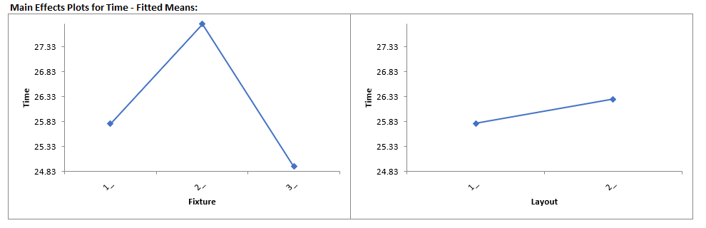
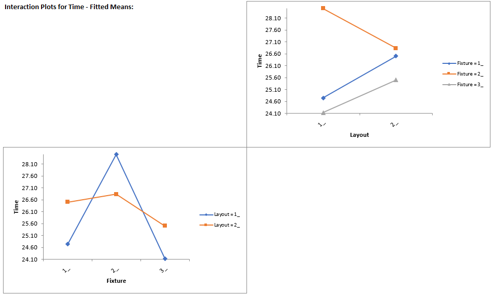
Click Sheet GLM1 - Plots to view the Main Effects and Interaction Plots.
Clearly Fixture 2 results in an increase in assembly time. This may be an operator training issue but possibly the fixture can be modified to help the operators perform the assembly task more quickly.
Note: The Main Effects and Interaction Plots are computed from the predicted values of the regression model which assumes that all factors are fixed. Confidence Intervals for the Main Effects plots are not available when there
is a Random Factor.