DiscoverSim™ Case Studies

Case Study 4 – Catapult Variation Reduction

Introduction: Optimizing Catapult Distance Firing Proces

This is an example of DiscoverSim stochastic optimization for catapult distance variation reduction, adapted from:

John O'Neill, Sigma Quality Management.

This example is used with permission of the author.

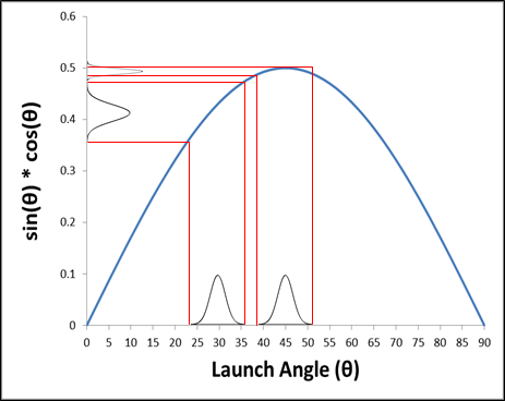
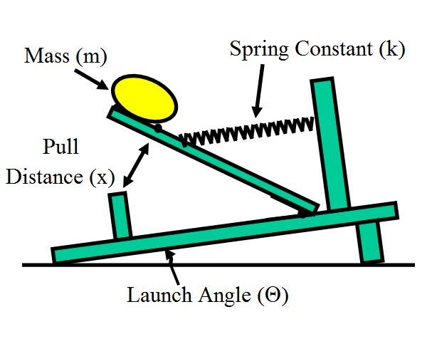
The figure below is a simplified view of the catapult:

The target catapult firing distance, Y = 50 +/- 2.5 feet.

To keep the model simple, only four factors (X’s) are included:

1. Spring Constant (k) – The spring constant is the force/foot required to pull back the catapult arm (in lbf/ft.). The initial parameters for this factor: normally distributed, mean of 47.3, standard deviation of 0.1.


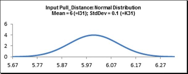
2. Pull Distance (x) – This is the distance in feet the arm is pulled back to launch the mass. The initial parameters for this factor: normally distributed, mean of 6.0, standard deviation of 0.1.


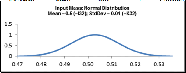
3. Mass (m) – This is the mass of the object in slugs (lbf/ft/sec^2). The initial parameters for this factor: normally distributed, mean of 0.5, standard deviation of 0.01.


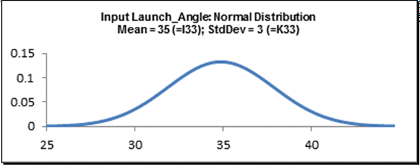
4. Launch Angle (θ) – This is the angle in degrees to the horizontal at which the mass leaves the catapult. The initial parameters for this factor: normally distributed, mean of 35, standard deviation of 3.
   
   Note: The degrees must be converted into radians for input to the Excel sine and cosine functions.

The Y = f(X) relationship is derived from conservation of energy and basic time, distance, acceleration relationships. Note that air resistance and other “real world” factors have been ignored to keep the model simple. Standard Gravity (g) is 32.174 ft/sec^2:

In this study we will use DiscoverSim to help us answer the following questions:

• What is the predicted process capability with these nominal settings?


• What are the key X variables that influence catapult firing distance Y?


• Can we adjust the nominal settings of X to reduce the transmitted variation in Y, thereby making the distance response robust to the variation in inputs?


• Can we further reduce the variation of the key input X’s in order to achieve an acceptable process capability?

Summary of DiscoverSim Features Demonstrated in Case Study 4:

Create Input Distributions (Continuous Normal) DiscoverSim Copy/Paste Cell Run Simulation with Sensitivity Chart of Correlation Coefficients Create Continuous Input Controls for Parameter Optimization Run Optimization

Catapult Simulation and Optimization with DiscoverSim

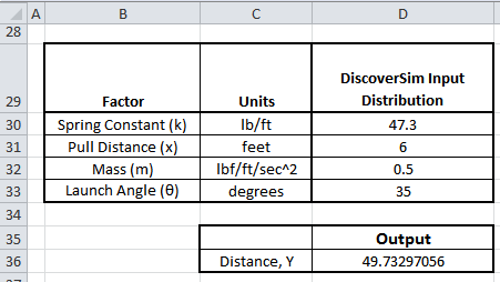
1. Open the workbook Catapult Model. DiscoverSim Input Distributions will simulate the variability in the catapult input factor X’s. We will specify the Normal Distribution for each X in cells D30 to D33. The output, Distance, will be specified at cell D36 using the formula given in the Introduction.
   
   


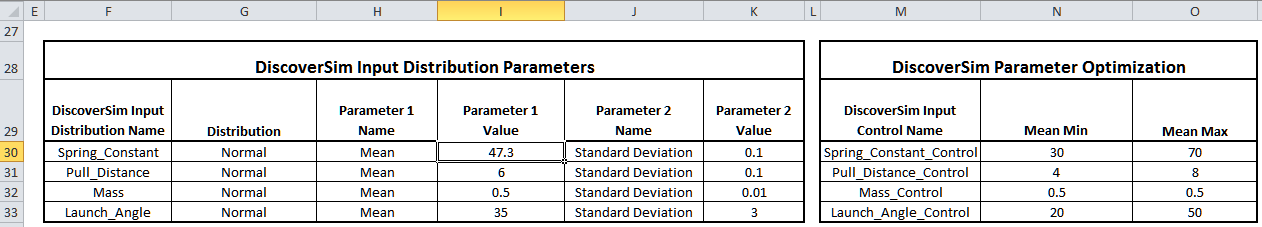
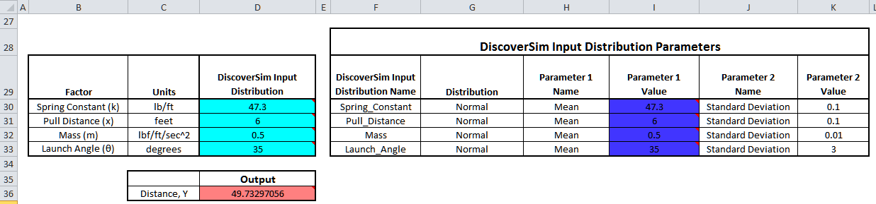
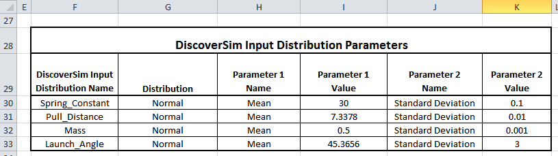
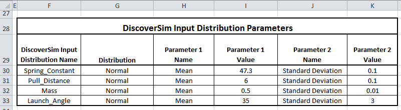
2. The Input Distribution parameters are given in the following table:
   
   


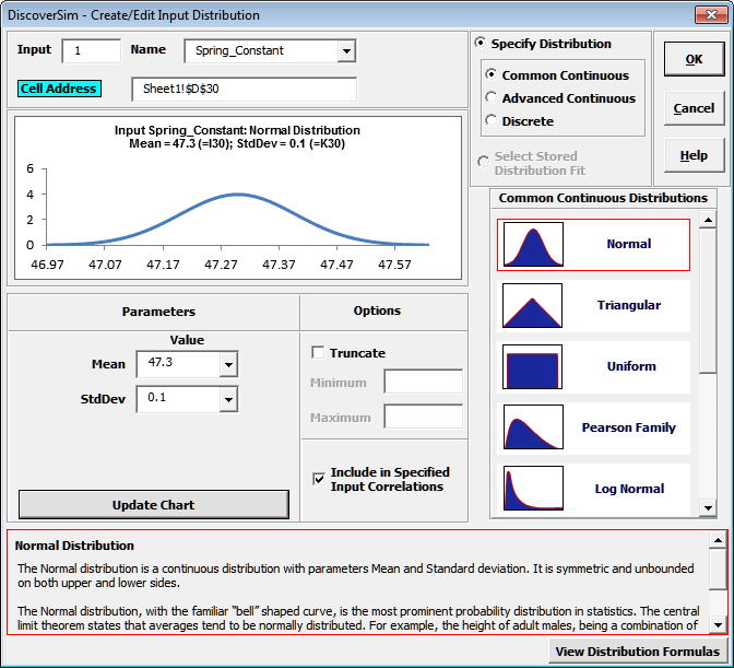
3. Click on cell D30 to specify the Input Distribution for X1, Spring Constant. Select DiscoverSim > Input Distribution:
   
   


4. We will use the selected default Normal Distribution.


5. Click input Name cell reference and specify cell F30 containing the input name “Spring_Constant”. After specifying a cell reference, the dropdown symbol changes from to .


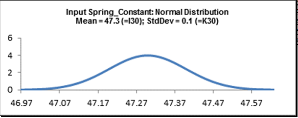
6. Click the Mean parameter cell reference and specify cell I30 containing the mean parameter value = 47.3.


7. Click the StdDev parameter cell reference and specify cell K30 containing the Standard Deviation parameter value = 0.1.


8. Click Update Chart to view the Normal Distribution as shown:
   
   


9. Click OK. Hover the cursor on cell D30 to view the DiscoverSim graphical comment showing the distribution and parameter values:
   
   


10. Click on cell D30. Click the DiscoverSim Copy Cell menu button (Do not use Excel’s Copy – it will not work!).


11. Select cells D31:D33. Now click the DiscoverSim Paste Cell menu button (Do not use Excel’s Paste – it will not work!).


12. Review the input comments in cells D31 to D33:



Cell D31






Cell D32






Cell D33





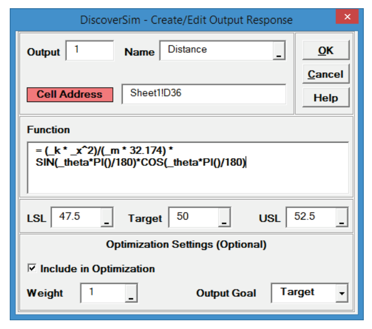
13. Click on cell D36. Note that the cell contains the Excel formula for Catapult Firing Distance. Excel range names are used rather than cell addresses to simplify interpretation.


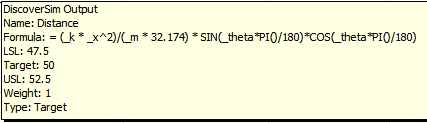
14. Select DiscoverSim > Output Response:
    
    


15. Enter the output Name as “Distance”. Enter the Lower Specification Limit (LSL) as 47.5, Target as 50, and Upper Specification Limit (USL) as 52.5.
    
    
    
    Click OK


16. Hover the cursor on cell D36 to view the DiscoverSim Output information.
    
    


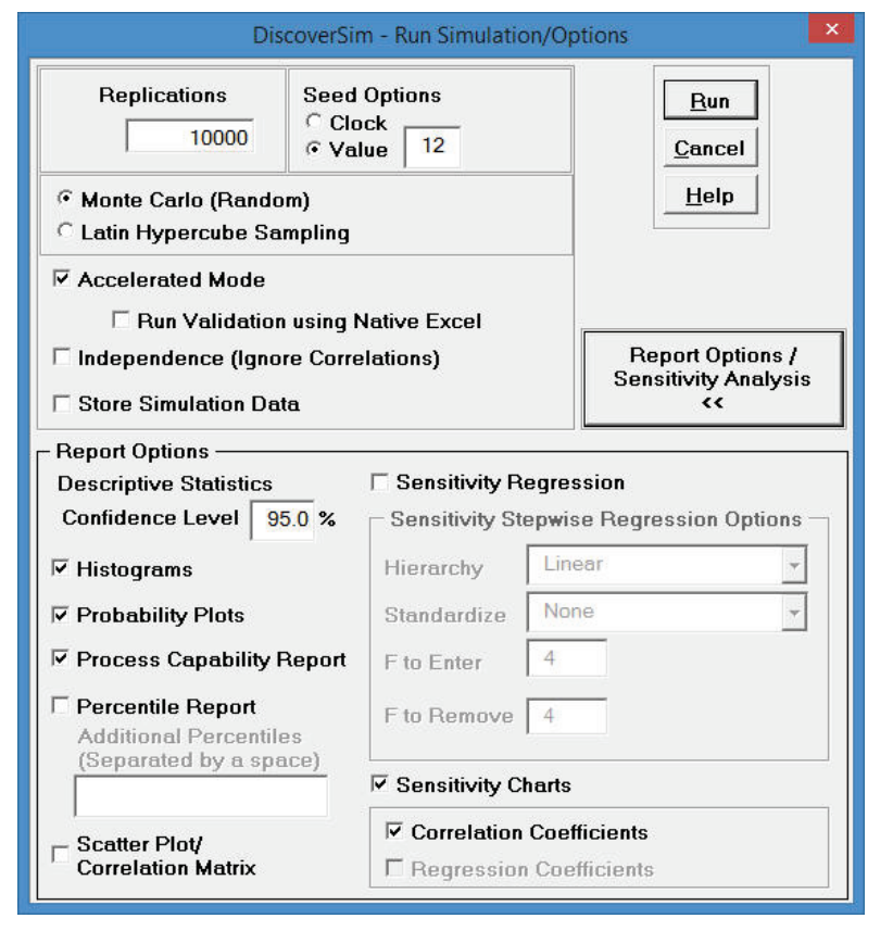
17. Select DiscoverSim > Run Simulation:
    
    


18. Click Report Options/Sensitivity Analysis. Check Sensitivity Charts and Correlation Coefficients. Select Seed Value and enter “12” as shown, in order to replicate the simulation results given below.
    
    
    
    Click Run.


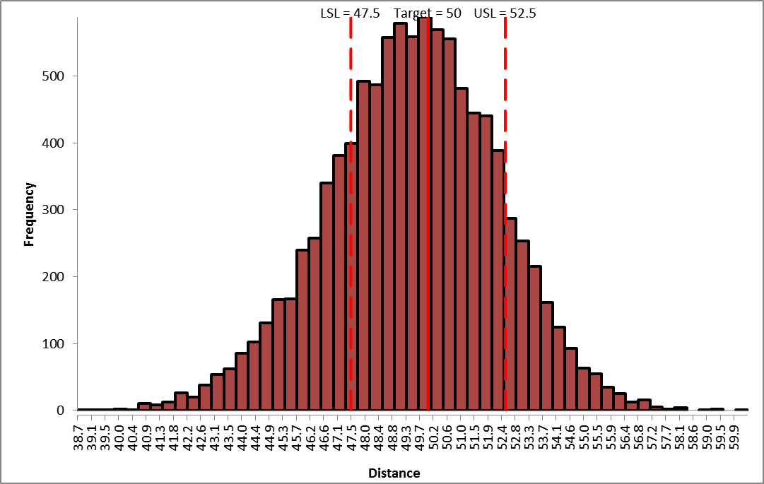
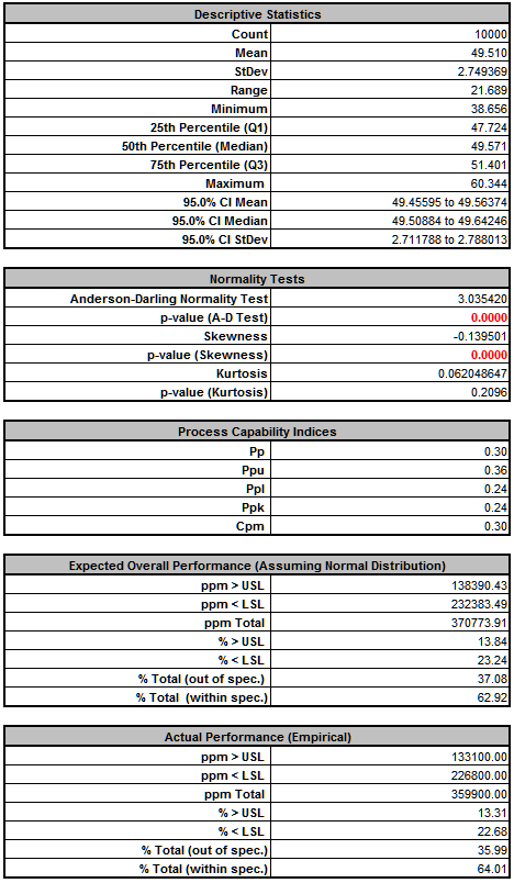
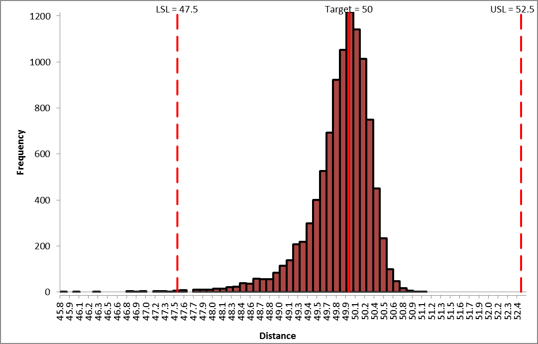
19. The DiscoverSim Output Report shows a histogram, descriptive statistics and process capability indices:
    
    
    
    From the histogram and capability report we see that the catapult firing distance is not capable of meeting the specification requirements. The variation is unacceptably large. Approximately 36% of the shots fired would fail, so we must improve the process to reduce the variation.
    
    Note: The output distribution is not normal (skewed left), even though the inputs are normal. This is due to the non-linear transfer function.


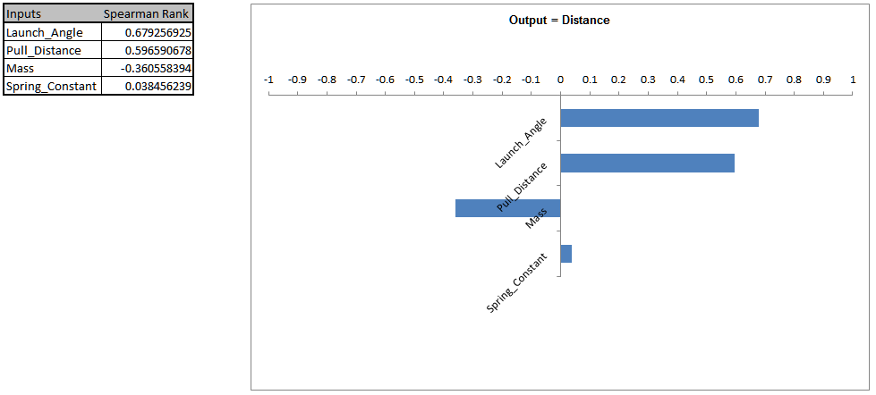
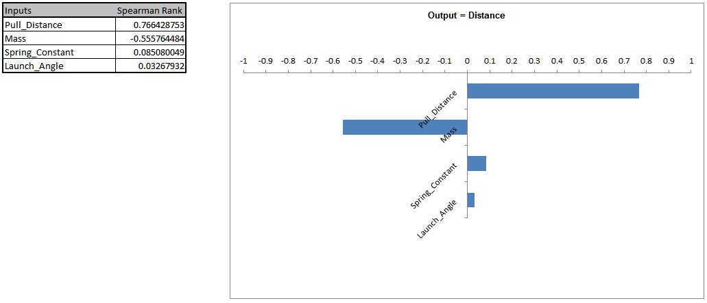
20. Click on the Sensitivity Correlations sheet:





Launch Angle is the dominant input factor affecting Distance, followed by Pull Distance. At this point we could put procedures in place to reduce the standard deviation of these input factors, but before we do that we will run optimization to determine if the process can be made robust to the input variation.



21. In order to perform parameter optimization, we will need to add Input Controls in cells I30 to I33. Select Sheet1. The Input Control parameters (min/max) are also shown below:




These controls will vary the nominal mean values for Spring Constant, Pull Distance and Launch Angle. Mass is kept fixed at 0.5. The standard deviation values will also be kept fixed for this optimization.



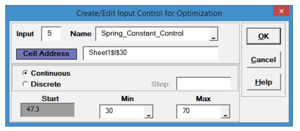
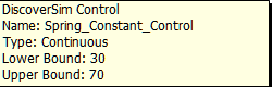
22. Click on cell I30. Select Control:
    
    


23. Click Input Name cell reference and specify cell M30 containing the input control name “Spring_Constant_Control”.


24. Click the Min value cell reference and specify cell N30 containing the minimum optimization boundary value = 30.


25. Click the Max value cell reference and specify cell O30 containing the maximum optimization boundary value = 70:
    
    


26. Click OK. Hover the cursor on cell I30 to view the comment displaying the input control settings:
    
    


27. Click on cell I30. Click the DiscoverSim Copy Cell menu button (Do not use Excel’s Copy – it will not work!).


28. Select cells I31:I33. Click the DiscoverSim Paste Cell menu button (Do not use Excel’s Paste – it will not work!).


29. Review the Input Control comments in cells I31 to I33.


30. The completed model is shown below:
    
    


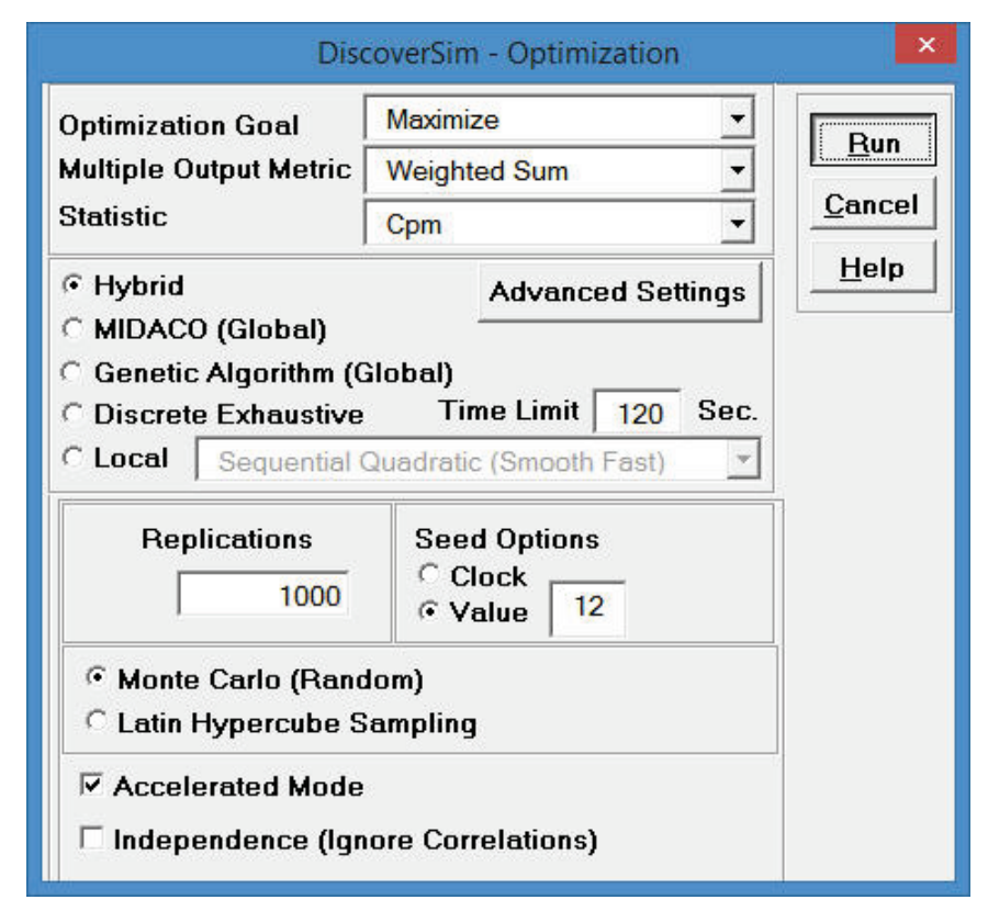
31. Now we are ready to perform the optimization. Select DiscoverSim > Run Optimization:
    
    


32. Select “Maximize” for Optimization Goal, “Weighted Sum” for Multiple Output Metric and “Cpm” for Statistic. Select Seed Value and enter “12” and Replications to 1000 in order to replicate the optimization results given below. All other settings will be the defaults as shown:
    
    
    
    Maximize Cpm is used here because it incorporates a penalty for mean deviation from target. We want the distance mean to be on target with minimal variation.
    
    We will use the Hybrid optimization method which requires more time to compute, but is very powerful to solve complex optimization problems.
    
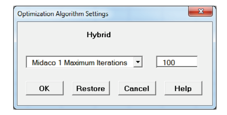
    Tip: To speed up this optimization, change the maximum number of iterations in Hybrid Midaco 1 (first MIDACO run) from 1000 to 100. Click Advanced Settings. Select Midaco 1 Maximum Iterations. Enter 100 as shown. Click OK.
    
    


33. Click Run.


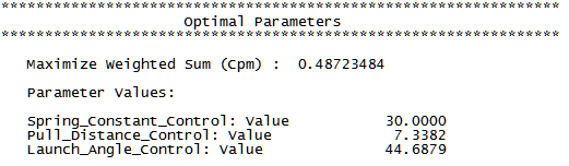
34. The final optimal parameter values are given as:
    
    
    
    The predicted Cpm value is 0.49, which is an improvement over the baseline value of 0.3.


35. You are prompted to paste the optimal values into the spreadsheet:
    
    
    
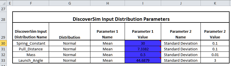
    Click Yes. This replaces the nominal Input Control values to the optimum values.
    
    
    
    Note that the expected values displayed in the Input Distributions are not automatically updated, but the new referenced Mean values will be used in simulation. To manually update the expected values and chart comments, click on each input cell, select Input Distribution and click OK.


36. Select Run Simulation. Click Report Options/Sensitivity Analysis. Check Sensitivity Charts and Correlation Coefficients. Select Seed Value and enter “12”, in order to replicate the simulation results given below Click Run.


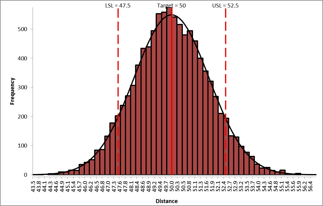
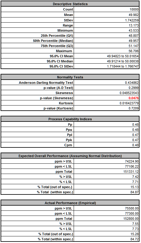
37. The resulting simulation report confirms the predicted process improvement:
    
    
    
    The standard deviation has been reduced from 2.75 to 1.74. The % Total (out-of-spec) has been decreased from 36.0% to 15.3%. This was achieved simply by shifting the mean input values so that the catapult transmitted variation is reduced. The key variable here is the launch angle mean shifting from 30 degrees to 45 degrees as illustrated in the simplified diagram below:
    
    
    
    Note: the illustrated improvement here is more dramatic than what was actually realized in the optimization due to the influence of the other input variables.


38. We will continue our improvement efforts, now focusing on reducing the variation of the inputs. Click on the Sensitivity Correlations (2) sheet:
    
    
    
    Pull Distance and Mass are now the dominant input factors affecting Distance.
    Note: Launch Angle now has the least influence due to the minimized transmitted variation at 45 degrees.


39. Select Sheet1, and change the standard deviation for Pull Distance from 0.1 to 0.01 (K31), and standard deviation for Mass from .01 to .001 (K32) as shown.
    
    
    
    Of course it is one thing to type in new standard deviation values to see what the results will be in simulation, but it is another to implement such a change. This requires updates to standard operating procedures, training of operators, tightening of component tolerances and likely increased cost. Robust parameter optimization, as demonstrated above, is easy and cheap. Reducing the variation of inputs can be difficult and expensive.


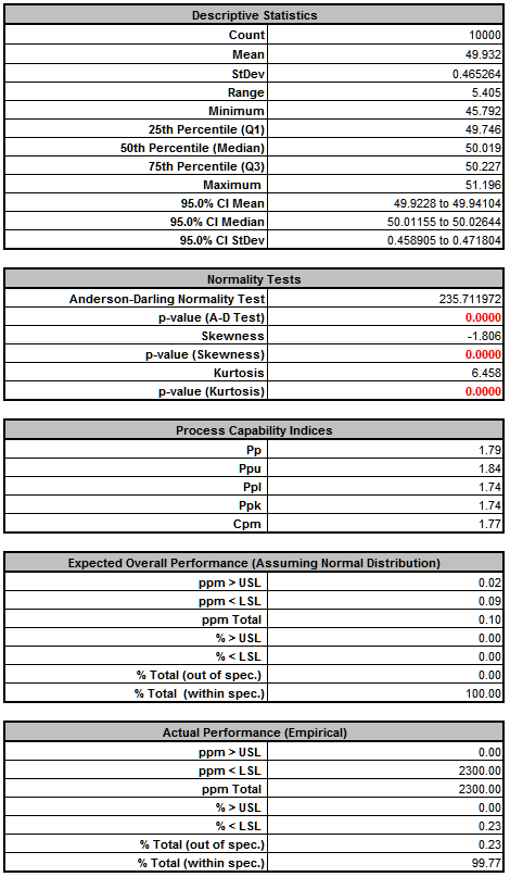
40. Select Run Simulation. Click Run. The resulting simulation report shows the further process improvement:
    
    
    
    The standard deviation has been further reduced from 1.74 to 0.47. The % Total (out-of-spec) has decreased from 15.3% to 0.2%.
    
    Note: The distribution is not normal (skewed left) due to the non-linearity in the transfer function.
    
    This is not yet a Six Sigma capable process, but it has been dramatically improved. Additional process capability improvement could be realized by optimizing %Ppk (Percentile based Ppk is best for non-normal distributions) rather than Cpm. This would shift the mean to the right of the target, to compensate for the skew left distribution, but the trade-off of mean being on target versus reduction in defects below the lower specification would need to be considered.