Difference Data

Utilities — Difference Data

Nonseasonal and Seasonal Differencing are used to make a process stationary. This is done automatically in ARIMA, but this utility makes it easy to do manually. This was demonstrated previously in the section Run Chart.

1. Open Chemical Process Concentration Series A.xlsx (Sheet 1 tab). This is the Series A data from Box and Jenkins, a set of 197 concentration values from a chemical process taken at two-hour intervals.


2. Click SigmaXL > Time Series Forecasting > Utilities > Difference Data. Ensure that the entire data table is selected. If not, check Use Entire Data Table. Click Next.


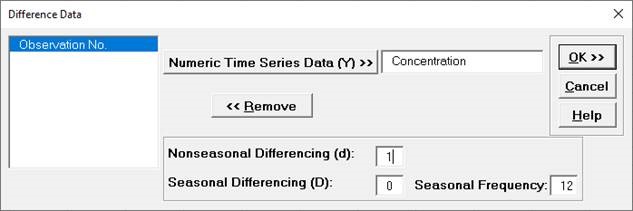
3. Click Concentration, click Numeric Time Series Data (Y) >>. Enter 1 for Nonseasonal Differencing (d).

   
   
   



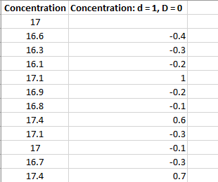
4. Click OK. A new sheet is created with the order d = 1 differenced data (Y₂ − Y₁, Y₃ − Y₂, …).
   
   
   
   This CCF plot shows significant cross correlation from lag = −9 to +9, with a peak at 0, however the autocorrelation in X and Y data is masking the true nature of the cross correlation.


5. Open Monthly Airline Passengers - Series G.xlsx (Sheet 1 tab). This is the Series G data from Box and Jenkins, monthly total international airline passengers for January 1949 to December 1960 and is one of the most popular datasets used in introductory time series forecasting.


6. Click the Sheet 1 tab. Click SigmaXL > Time Series Forecasting > Utilities > Difference Data. Ensure that the entire data table is selected. If not, check Use Entire Data Table. Click Next.
   


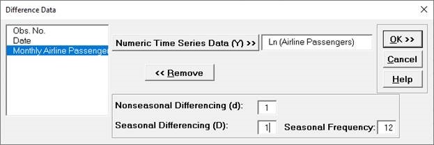
7. Select Ln(Airline Passengers), click Numeric Time Series Data (Y)>>. Enter 1 for Nonseasonal Differencing (d); enter 1 for Seasonal Differencing (D); Seasonal Frequency is specified as 12.
   
   
   


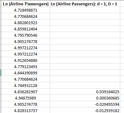
8. Click OK. A new sheet is created with the seasonal order D = 1 differenced data (Y₁₃ − Y₁, Y₁₄ − Y₂, …) and nonseasonal order d=1 (D₂ − D₁, D₃ − D₂, …).