Include Top

Design and Analysis of Catapult Full Factorial Experiment


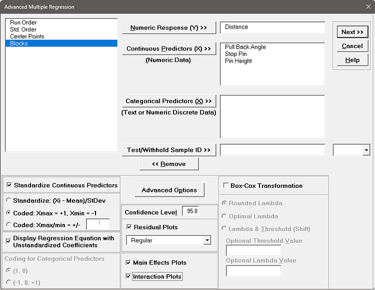
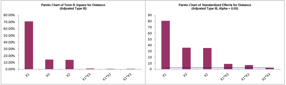
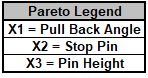
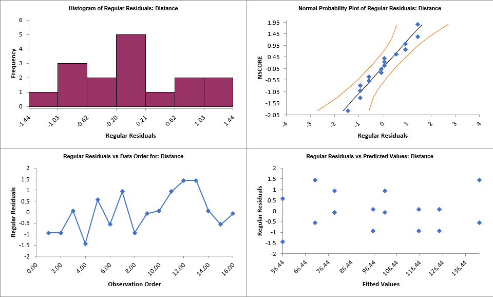
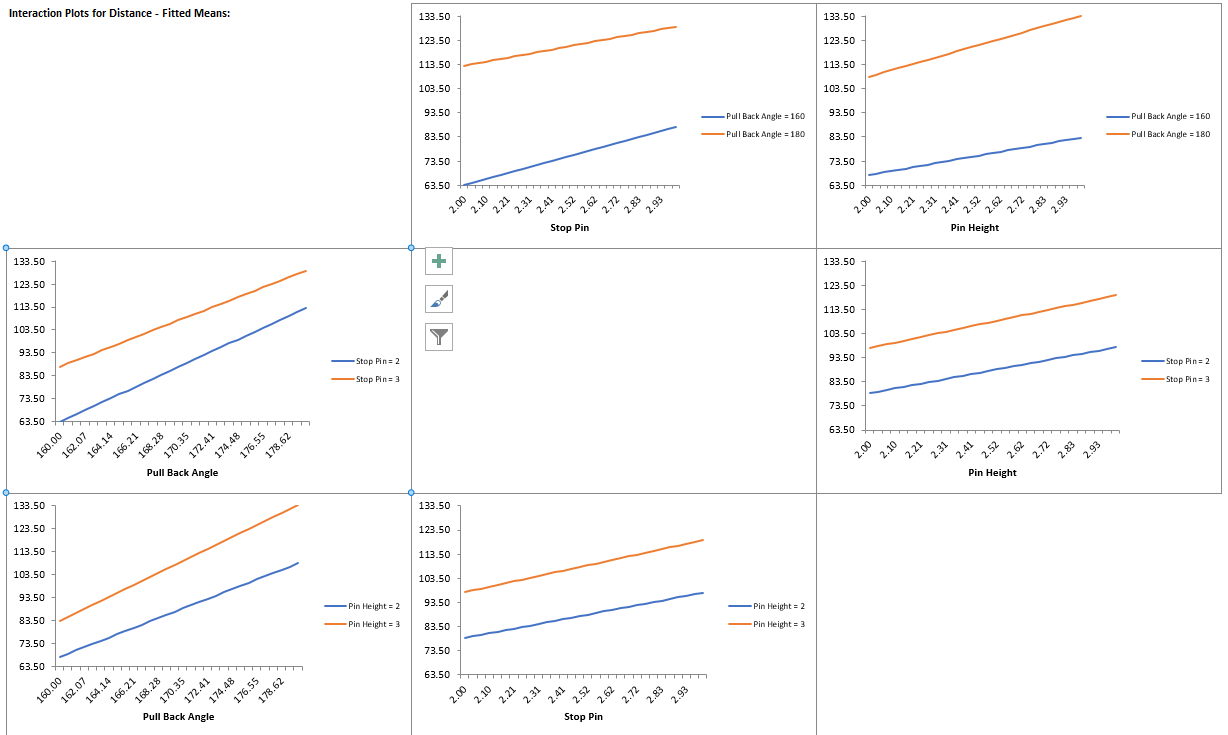
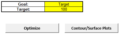
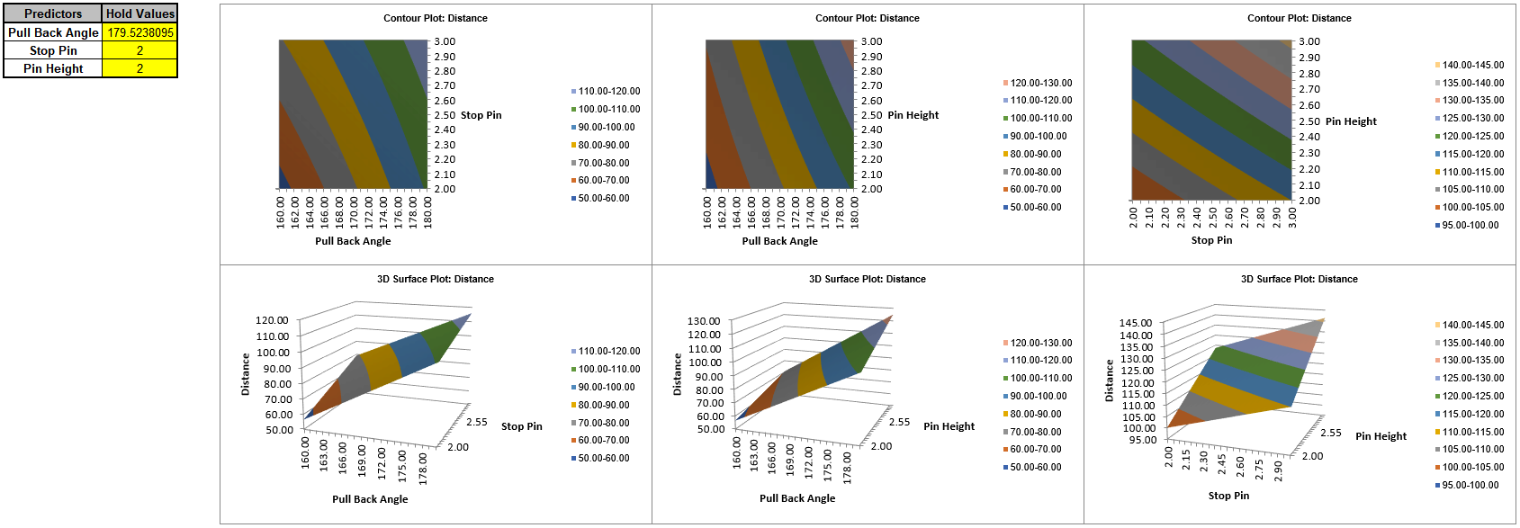
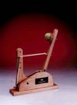
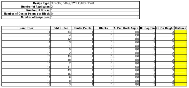
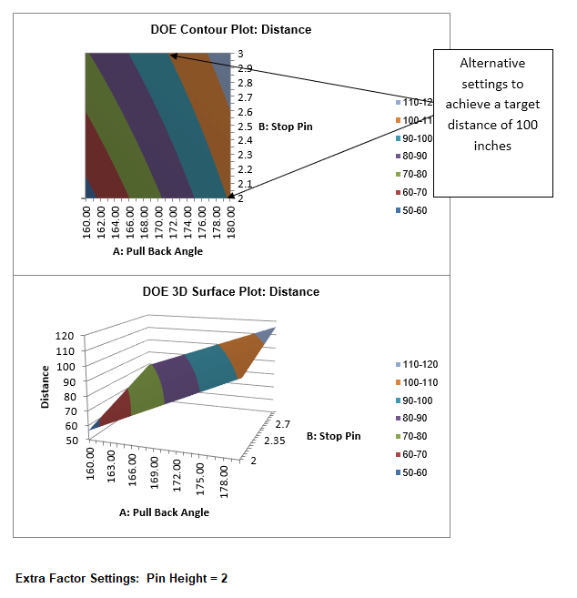
Catapults are frequently used in Six-Sigma or Design of Experiments training. They are a powerful teaching tool and make the learning fun. If you have access to a catapult, we recommend that you perform the actual experiment and use your own data. Of course, you can also follow along using the data provided. The response variable (Y) is distance, with the goal being to consistently hit a target of 100 inches.

  1. Click SigmaXL > Design of Experiments > 2-Level Factorial/Screening > 2-Level Factorial/Screening Designs.

  2. The Number of X Factors can be 2 to 19. Using process knowledge, we will limit ourselves to 3 factors: Pull Back Angle, Stop Pin and Pin Height. Pull Back will be varied from 160 to 180 degrees, Stop Pin will be positions 2 and 3 (count from the back), and Pin Height will be positions 2 and 3 (count from the bottom).

  3. Select Number of Factors = 3.

  4. The available designs are then given as: 4-Run, 2**(3-1), 1/2 Fraction, Res III and 8-Run, 2**3, Full-Factorial. If we had more than 5 factors, a Resolution III or Plackett-Burman Screening design would typically be used. Here we will choose the 8-Run, 2**3, Full-Factorial design.

    2 Level Factorial Design of Experiments

    Notes: Design Generators and Aliasing of Effects will be reported for Fractional Factorial designs. When the Number of Factors is 9 or higher, Factor Name “I” is not used, in order to avoid confusion with the Fractional Factorial Defining Relation “I”.

    The Power Information is presented to assist the user with selection of number of runs and replicates for the design, so that one can see the trade-off between experimental cost and sensitivity to detect Effects of interest.

    Power (1-Beta) < 0.5 is considered as Very Low Power to detect Effect.
    Power (1-Beta) >= 0.5 and < 0.8 is considered as Low Power to detect Effect.
    Power (1-Beta) >= 0.8 and < 0.95 is considered as Medium Power to detect Effect.
    Power (1-Beta) >= 0.95 and < 0.99 is considered as High Power to detect Effect.
    Power (1-Beta) >= 0.99 is considered as Very High Power to detect Effect.

    The power calculations require an estimate of experimental error, so when Replicates = 1 an assumption of 3 center points is used in order to give an approximate reference level of power (regardless of the value for Number of Center Points per Block).

  5. This design currently shows the following:

    These power calculations assume 3 center points:
    Very Low Power to detect Effect = 1*StDev (1-Beta < 0.5);
    Very Low Power to detect Effect = 2*StDev (1-Beta < 0.5);
    Medium Power to detect Effect = 3*StDev (0.8 <= 1-Beta < 0.95).

    We would like to have medium power to detect an Effect = 2*StDev.
    Change the Number of Replicates to 2. The Power Information is now:
    Very Low Power to detect Effect = 1*StDev (1-Beta < 0.5);
    Medium Power to detect Effect = 2*StDev (0.8 <= 1-Beta < 0.95);
    Very High Power to detect Effect = 3*StDev (1-Beta >= 0.99).
    We will therefore choose two replicates. The number of replicates will always be a tradeoff between the desired power and the cost of the experimental runs.

    Specify 2 or more blocks if there are constraints such as the number of runs per day or some other known external “nuisance” variable (like 2 different catapults or 2 operators). Here we will keep Blocks = 1 (i.e., no Blocking).

    Center Points are useful to provide an estimate of experimental error with unreplicated designs, and allow detection of curvature. Typically 3 to 5 center points are used. Here we will not use center points because we have replicated the design twice and do not expect significant curvature in the distance response. Furthermore, center points could not be set for Pin Height and Stop Pin (without drilling additional holes!).

  6. Complete the Factor Names, Level Settings and Response Name as shown:

    2 Level Factorial Design of Experiments

  7. Click OK. The following worksheet is produced:

  8. Design of Experiments Worksheet

  9. You can enter information about the experiment in the fields provided. If you have access to a catapult, perform the experimental runs in the given randomized sequence, and enter the distance values in the Distance column.

  10. If you are not able to perform the catapult experiment, open the file Catapult DOE V6.xlsx.

  11. Before we begin the regression analysis, we will have a quick look at the Main Effects and Interaction Plots. Click SigmaXL > Design of Experiments > 2 Level Factorial/Screening Main Effects & Interaction Plots. The resulting plots are shown below:

  12. interaction plots

    Pull Back Angle is the dominant factor having the steepest slope. We can also see that the interaction terms are weak with the almost parallel lines.

  13. Click SigmaXL > Design of Experiments > 2-Level Factorial/Screening > Analyze 2-Level Factorial/Screening Design.

  14. Analyze 2 Level Factorial Design of Experiments

  15. We will use the default analyze settings (all terms in the model) to start. Click OK. The resulting Analysis report is shown:

    Design of Experiments Analysis
    Pareto Chart

  16. The model looks very good with an R-Square value of 99.9%! The standard deviation (experimental error) is only 1.03 inches. Clearly Pull Back Angle is the most important predictor (X factor), but all the main effects and two-way interaction are significant. However, the three-way interaction is not significant, so it should be removed from the model.

  17. Click Recall Last Dialog (or press F3).

  18. Remove the ABC interaction term as shown:

    2 Level Factorial Design of Experiments

  19. Click OK. The revised report is shown below:

  20. DOE Analysis

    Pareto Chart

  21. All the terms in the model are now significant, and there is no evidence of lack of fit (P-value for lack-of-fit is 0.128 which is > .05).

  22. Scroll down to view the Residual Plots. They also look very good, approximately normal, with no obvious patterns:

  23. Residuals Plots

  24. Scroll up to the Predicted Response Calculator. Enter the predicted values shown. These initial settings were determined by trial and error.

  25. Predicted Response Calculator

    Note: CI is the 95% confidence interval for the long term mean and PI is the 95% prediction interval for individual values.

    Note: The DOE Multiple Regression Model: Distance equation given above uses the coded coefficients, so if this equation is used to do predictions, the inputs must first be coded as done in the Predicted Response Calculator.

  26. Excel’s Solver may also be used to get a more exact solution:

    Excel Solver

  27. The model prediction must then be confirmed with actual experimental runs at the given settings of Pull Back Angle = 179.5, Stop Pin = 2, and Pin Height = 2.

  28. Alternative settings to achieve the target distance may be obtained with Contour/Surface Plots. Click SigmaXL > Design of Experiments > 2-Level Factorial/Screening > Contour/Surface Plots. Set the Pin Height to 2 as shown (after clicking OK, you can use Recall SigmaXL Dialog to create another Contour/Surface plot with Pin Height set to 3):

    Contour Surface Plots

  29. Click OK. The following Contour and Surface Plots are displayed (with Pin Height = 2). Note the contour line with Catapult target distance = 100 inches. Although pin settings are discrete, they appear as continuous, so this will be a constraint in our selection of alternative settings. In addition to Pull Back Angle = 179.5, Stop Pin = 2, Pin Height = 2, we see that Pull Back Angle approx. = 171, Stop Pin = 3, Pin Height = 2 is also a valid setting. Alternative setting options are valuable in a designed experiment because they allow you to select lowest cost optimum settings, or settings that are easier to control.

  30. Contour Surface Plots

    Tip: Use the contour/surface in conjunction with the predicted response calculator to determine optimal settings.

Analysis of Catapult Full Factorial Experiment with Advanced Multiple Regression


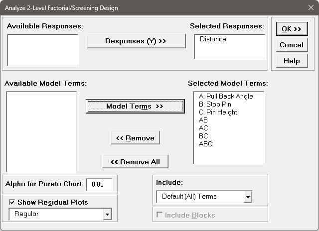
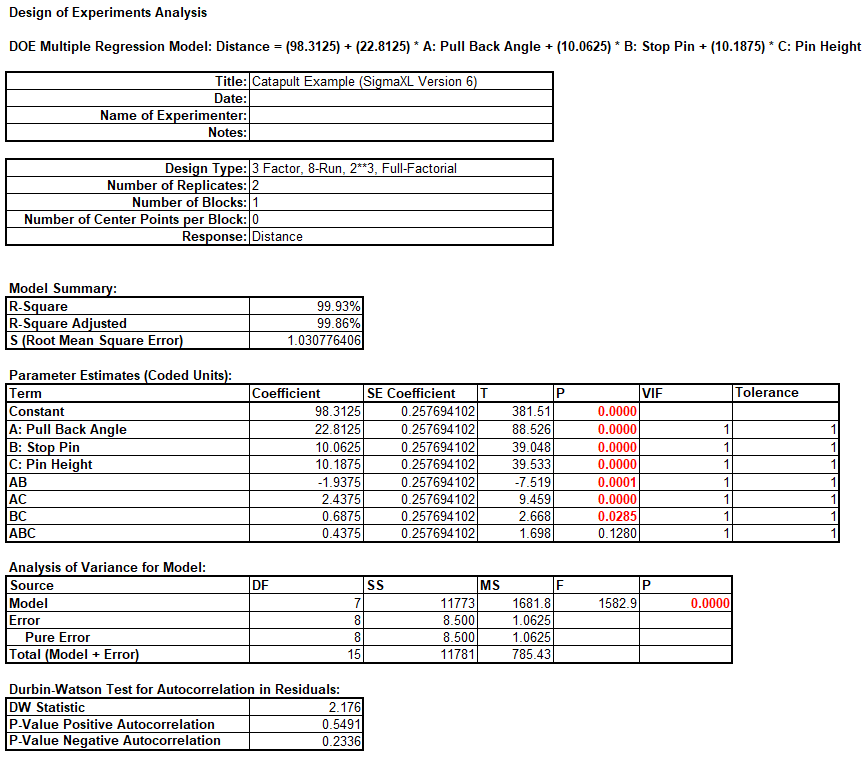
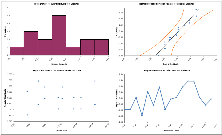
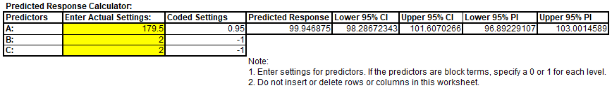
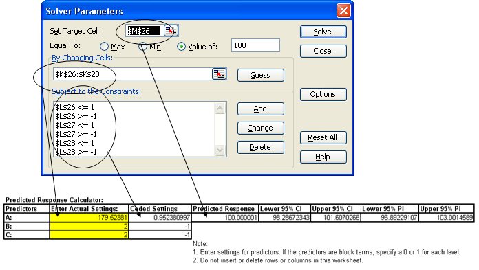
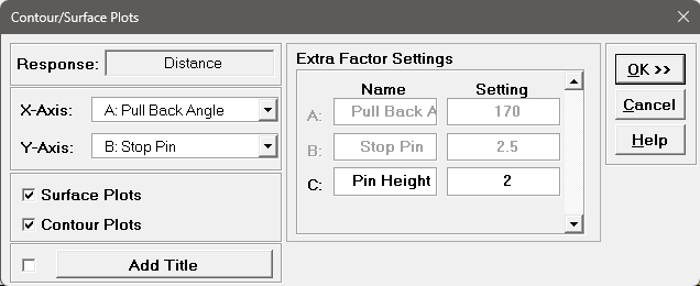
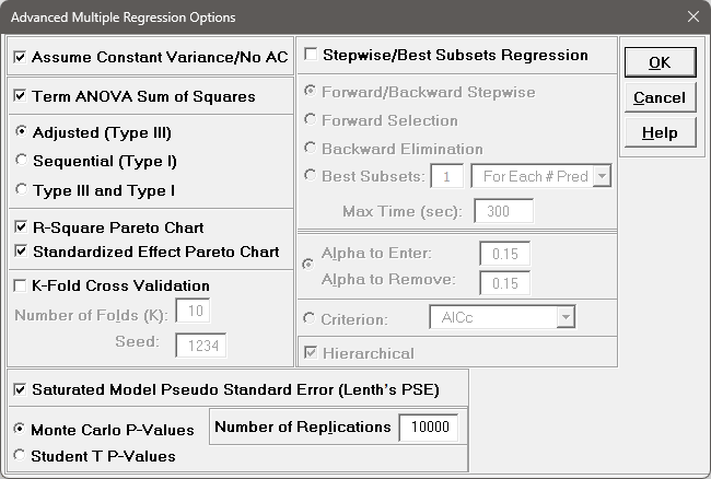
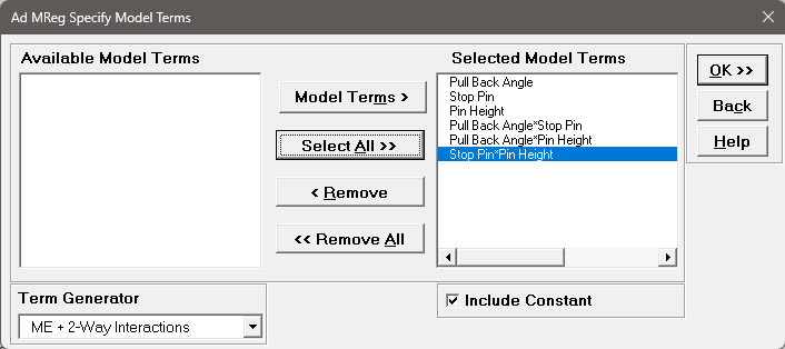
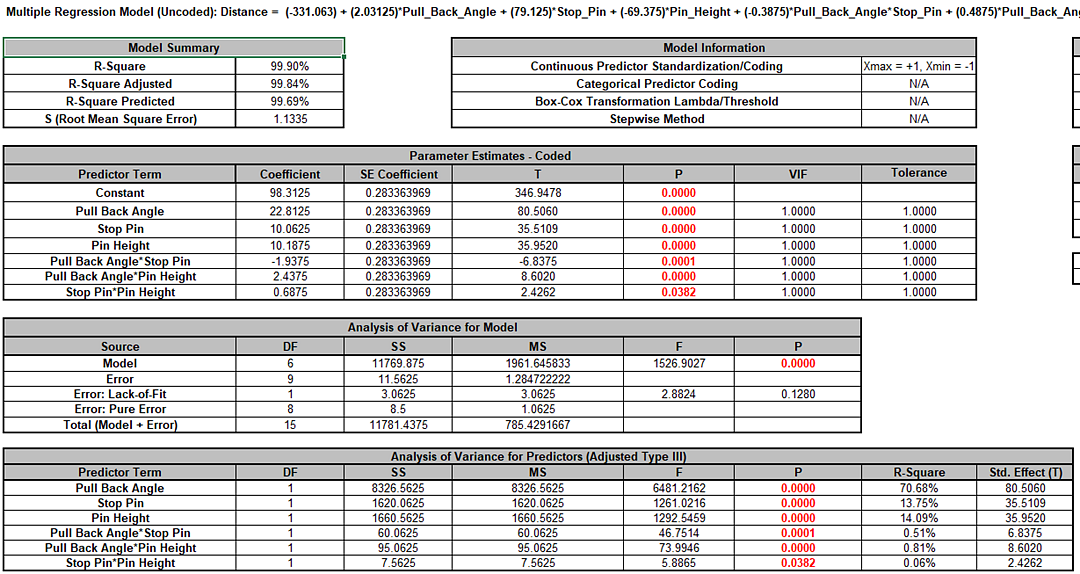
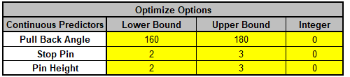
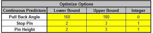
We will now redo the above analysis and optimization using Advanced Multiple Regression.


  1. Open the file Catapult DOE Data for Adv MReg.xlsx. This is the Catapult DOE data copied into a workbook with A:, B: and C: removed from the Factor Names as they are not needed for Advanced Multiple Regression.

  2. Click Sheet 1 Tab. Click SigmaXL > Statistical Tools > Advanced Multiple Regression > Fit Multiple Regression Model. If necessary, click Use Entire Data Table, click Next.

  3. Select Distance, click Numeric Response (Y) >>; select Pull Back Angle, Stop Pin, and Pin Height; click Continuous Predictors (X) >>. Check Standardize Continuous Predictors with option Coded: Xmax = +1, Xmin = -1. Check Display Regression Equation with Unstandardized Coefficients. Use the default Confidence Level = 95.0%. Regular Residual Plots are checked by default. Check Main Effects Plots and Interaction Plots. Leave Box-Cox Transformation unchecked.

    Advanced Multiple Regression Catapult Model Settings

    • Standardize Continuous Predictors with Coded: Xmax = +1, Xmin = -1 scales the continuous predictors so that Xmax is set to +1 and Xmin is set to -1. This is particularly useful for analyzing data from a factorial design of experiments as we are doing here.

    • Display Regression Equation with Unstandardized Coefficients displays the prediction equation with unstandardized/uncoded coefficients but the Parameter Estimates table will still show the standardized coefficients. This format is easier to interpret since there is only one coefficient value for each predictor.

  4. Click Advanced Options. We will use the defaults as shown. Ensure that Stepwise/Best Subsets Regression is unchecked.

    Ad MReg Catapult Advanced Options

    • Term ANOVA Sum of Squares with Adjusted (Type III) provides a detailed ANOVA table for continuous and categorical predictors. Adjusted Type III is the reduction in the error sum of squares (SS) when the term is added to a model that contains all the remaining terms.

    • R-Square Pareto Chart displays a Pareto chart of term R-Square values (100*SSterm/SStotal). A separate Pareto Chart is produced for Type III and Type I SS. If there is only one predictor term, a Pareto Chart is not displayed.

    • Standardized Effect Pareto Chart displays a Pareto chart of term T values (=T.INV(1-P/2,dferror)). A separate Pareto Chart is produced for Type III and Type I SS. A significance reference line is include (=T.INV(1-alpha/2,dferror)).

    • Saturated Model Pseudo Standard Error (Lenth’s PSE) is checked by default, but is not used here, as this is only applicable to saturated models with 0 error degrees of freedom.

  5. Click OK. Using Term Generator, select ME + 2-Way Interactions. Click Select All >>. Include Constant is checked by default.

    Ad MReg Catapult Model Terms

    This matches the final model used in the original analysis for Distance. If we wanted to include the 3-Way Interaction, then ME + All Interactions would have been selected.

  6. Click OK. The Advanced Multiple Regression report for Distance is given:

    Ad MReg Catapult Report

    Ad MReg Catapult Pareto

    Ad MReg Catapult Pareto Legend

    Note, the prediction equation is uncoded so the coefficients do not match the coded coefficients given in the Parameter Estimates table. If consistency is desired, one can always rerun the analysis with Display Regression Equation with Unstandardized Coefficients unchecked. Blanks and special characters in the predictor names of the equation are converted to the underscore character “_”.

    The model summary statistics match the previous analysis. R-Square Predicted = 99.69%, also known as Leave-One-Out Cross-Validation, indicates how well a regression model predicts responses for new observations and is typically less than R-Square Adjusted. This is also very good.

    The Parameter Estimates and ANOVA match the previous analysis. The Pareto Chart of Standardized Effects for Distance with significance line is similar to the Pareto Chart of Abs(Coefficient) but is based on the term T statistic.

    Since this is an orthogonal design, Adjusted (Type III) Sum-of-Squares are the same as Sequential (Type I) Sum-of-Squares (not shown), so the Term R-Square Pareto shows the percent contribution to variabity in the Distance and sums to R-Square = 99.9%.

  7. The Durbin-Watson Test for Autocorrelation in Residuals table is:

    Ad MReg Catapult DW table

    The Durbin Watson (DW) test is used to detect the presence of positive or negative autocorrelation in the residuals at Lag 1. If either P-Value is < .05, then there is significant autocorrelation. Here, there is no significant autocorrelation in the residuals, which is what we would expect in a randomized design of experiments.

  8. The Breusch-Pagan Test for Constant Variance is:

    Breusch-Pagan Table

    There are two versions of the Breusch-Pagan (BP) test for Constant Variance: Normal and Koenker Studentized – Robust. SigmaXL applies an Anderson-Darling Normality test to the residuals in order to automatically select which version to use. If the AD P-Value < 0.05, Koenker Studentized – Robust is used.

    The report includes the test for All Terms and for individual predictors. All Terms denotes that all terms are in the model. This should be used to decide whether or not to take corrective action. The individual predictor terms are evaluated one-at-a-time and provide supplementary information for diagnostic purposes. Note, this should always be used in conjunction with an examination of the residual plots.

    Here we see that the All Terms test is not significant, so we conclude that the variance is constant.

    Tip: If the All Terms test is significant after model refinement, try a Box-Cox transformation. If that does not work, refit the model using Recall Last Dialog, click Advanced Options in the Advanced Multiple Regression dialog, and uncheck Assume Constant Variance/No AC. SigmaXL will apply the White robust standard errors for non-constant variance. For details, see the Appendix: Advanced Multiple Regression.

    Tip: Lack of Constant Variance (a.k.a. Heteroskedasticity) is a nuisance for regression modelling but is also an opportunity. Examining the residual plots and individual predictors may yield process knowledge that identifies variance reduction opportunities.

  9. Click on Sheet MReg1 – Residuals to view the Residual Plots. Note, Sheet MReg# will increment every time a model is refitted.

    Catapult Model - Advanced Multiple Regression Residual ChartsA

    Catapult Model - Advanced Multiple Regression Residual ChartsB

    Catapult Model - Advanced Multiple Regression Residual ChartsC

    The Residual Plots are similar to those in the previous analysis and look very good, approximately normal, with no obvious patterns.

    Note: Residuals versus interaction terms are not plotted, but they can be manually created using the model design matrix to the right of the Residual Plots (use SigmaXL > Graphical Tools > Scatter Plots).

  10. Click on Sheet MReg1 – Plots. The Main Effects Plots and Interaction Plots for Overall Satisfaction are shown.

    Catapult Model - Advanced Multiple Regression Interaction PlotsA

    Catapult Model - Advanced Multiple Regression Interaction PlotsB

    These are based on Fitted Means as predicted by the model, not Data Means as used in the previous analysis. Main Effects Plots with Fitted Means use the predicted value for the response versus input predictor value, while holding all other variables at their respective means. Similarly for Interaction Plots, all predictors not being plotted are held at their respective means.

    Pull Back Angle is the dominant factor having the steepest slope. We can also see that the interaction terms are weak with the almost parallel lines.

  11. Click on Sheet MReg1 – Model. Scroll to the Predicted Response Calculator. Enter Pull Back Angle = 179.5, Stop Pin = 2, Pin Height = 2 to predict Overall Satisfaction with the 95% confidence interval for the long term mean and 95% prediction interval for individual values:

    Catapult Model - Response Calculator

    Note the formula at cell L14 is an Excel formula.

    This matches the previous initial settings. Here the full predictor names are used making it easier to use and interpret. The Coded Settings are calculated as part of the Excel formula. Also, the prediction standard error SE is given.

  12. Next, we will use SigmaXL’s built in Optimizer. Scroll to view the Optimize Options:

    Catapult Model - Optimize OptionsA

    Here we can constrain the lower and upper bounds of the continuous predictors. (If there was a categorical predictor, e.g., different ball type, you could also specify a ball type to use for optimization). Stop Pin and Pin Height are constrained to integers so these should be changed from 0 to 1 as shown.

    Catapult Model - Optimize OptionsB

    The Optimizer will return only integer values for Stop Pin and Pin Height.

  13. Scroll back to view the Goal setting and Optimize button. Specify Target = 100 as shown.

    Catapult Model - Response Calculator Target=100

    The optimizer uses Multistart Nelder-Mead Simplex to solve for the desired response goal with given constraints. For more information see the Appendix: Single Response Optimization.

  14. Click Optimize. The response solution and prompt to paste values into the Input Settings of the Predicted Response Calculator is given:

    Catapult Model - Optimization Results 1

  15. Click Yes to paste the values.

    Catapult Model - Optimization Results Paste 1

  16. Scroll to view the Optimize Options, and change the Stop Pin Lower Bound = 2, Upper Bound = 2; Pin Height Lower Bound = 2, Upper Bound = 2 as shown:

    Catapult Model - Optimize Options 2

  17. Click Optimize. The response solution and prompt to paste values into the Input Settings of the Predicted Response Calculator is given:

    Catapult Model - Optimization Results 2

  18. Click Yes to paste the values.

    Catapult Model - Optimization Results Paste 2

    This now matches the Solver solution obtained in the previous analysis. Note however that the SE for the original SigmaXL solution is lower than the Solver solution. This is by design, when multiple valid solutions are available, SigmaXL selects the one with the lowest prediction SE.

  19. Next, we will create a Contour/Surface Plot. Click the Contour/Surface Plots button. Note that Stop Pin and Pin Height are not constrained to be integers in these plots.

  20. A new sheet is created, MReg1 – Contour that displays the plots:

    Catapult Model - Contour Plots ADMReg

    SigmaXL automatically creates a Contour/Surface Plot for each pairwise combination of continuous predictors. The plots on the left match those specified in the previous analysis.

    Note that the table with the Hold Values gives the values used to hold a predictor constant if it is not in the plot.

    Tip: The hold values are obtained from the Predicted Response Calculator settings, so if you wish to use different Hold Values, simply select the Model sheet, change the Enter Settings values and recreate the plots.

    Tip: Use the contour/surface plots in conjunction with the predicted response calculator to determine optimal settings.

Define, Measure, Analyze, Improve, Control

Lean Six Sigma Software Excel Add-in

Simulate, Optimize,
Realize

Lean Six Sigma Software Excel Add-in

Web Demos

Our CTO and Co-Founder, John Noguera, regularly hosts free Web Demos featuring SigmaXL and DiscoverSim
Click here to view some now!

Contact Us

Phone: 1.888.SigmaXL (744.6295)

Support: Support@SigmaXL.com

Sales: Sales@SigmaXL.com

Information: Information@SigmaXL.com