Design and Analysis of Response Surface Experiment Cake Bake
We will illustrate the use of response surface methods using a layer cake baking
experiment. The response variable is Taste Score (on a scale of 1-7 where 1 is "awful"
and 7 is "delicious"). Average scores for a panel of tasters have been recorded. The X
Factors are A: Bake Time (20 to 40 minutes) and B: Oven Temperature (350 to 400 F). The
experiment goal is to find the settings that maximize taste score. Other factors such as
pan size need to be taken into consideration. In this experiment, these are held
constant.
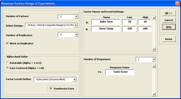
The Number of X Factors can be 2 to 5. Select Number of
Factors = 2.
The available designs are sorted by number of runs. Increasing the
number of runs allows for uniform precision or blocking, but we will select the design
with fewest runs, the 10-Run, Central Composite Design (2 Ctr Pts).
As discussed earlier with the catapult experiment, it is a good
practice to replicate an experiment if affordable to do so. Here we will select
Number of Replicates = 2 and check Block on
Replicates. Blocking on replicates allows us to perform the experiment over
a two week period, with each block corresponding to week number.
Change the Alpha Axial Value option to
Face Centered (Alpha = 1.0). This simplifies the design to a 3-level
design, rather than a 5-level design with alpha = 1.414. (The trade-off is that we lose
the desirable statistical property of rotatability for prediction).
Tip: This alpha is the distance from the center point to the end of
the axial (star) point. Do not confuse this with
Alpha for Pareto Chart which is the P-Value used to determine
statistical significance. Unfortunately, the term alpha has been chosen by
statisticians to define two completely different things.
Enter Factor Names and Level Settings and
Response Name as shown:
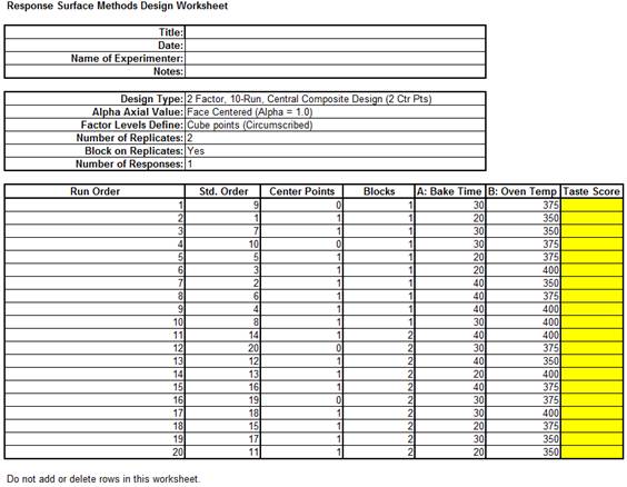
Click OK. The following worksheet is
produced:
Open the file RSM Example Cake Bake to obtain response values.
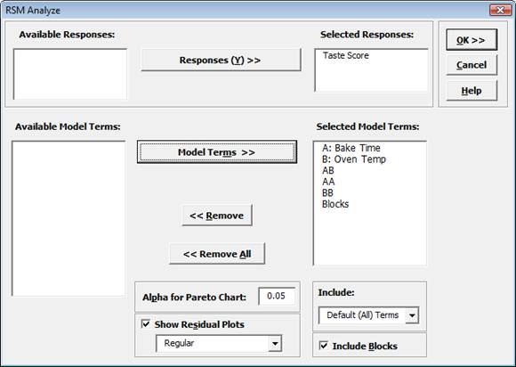
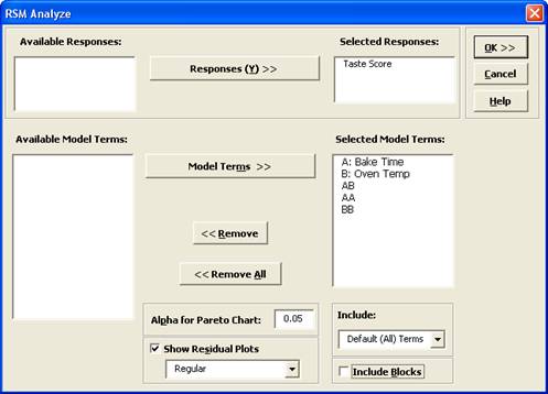
We will use the default analyze settings (all terms in the model, including the block
term) to start. Click OK. The resulting Analysis report is shown:
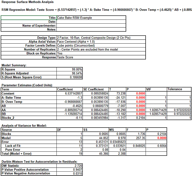
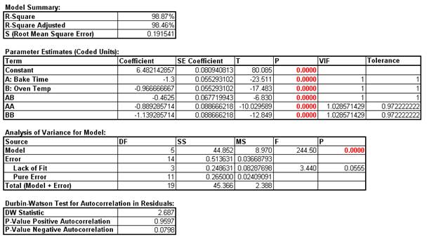
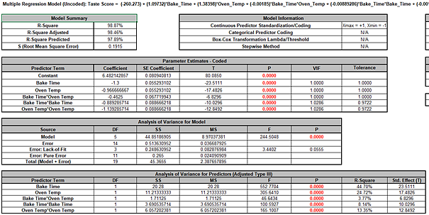
The model looks very good with an R-Square value of 99.0% The standard deviation
(experimental error) is only 0.19 on a 1 to 7 taste scale. All of the model terms are
statistically significant (P < .05), but the Block term is not, so it should be
removed from the model. Note that AA and BB denote the quadratic model terms.
Click Recall Last Dialog (or press F3).
Uncheck Include Blocks as shown:
Click OK. The revised report is shown below:
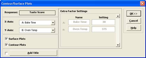
To create a contour and surface plot, click SigmaXL > Design of Experiments
> Response Surface > Contour/Surface Plots.
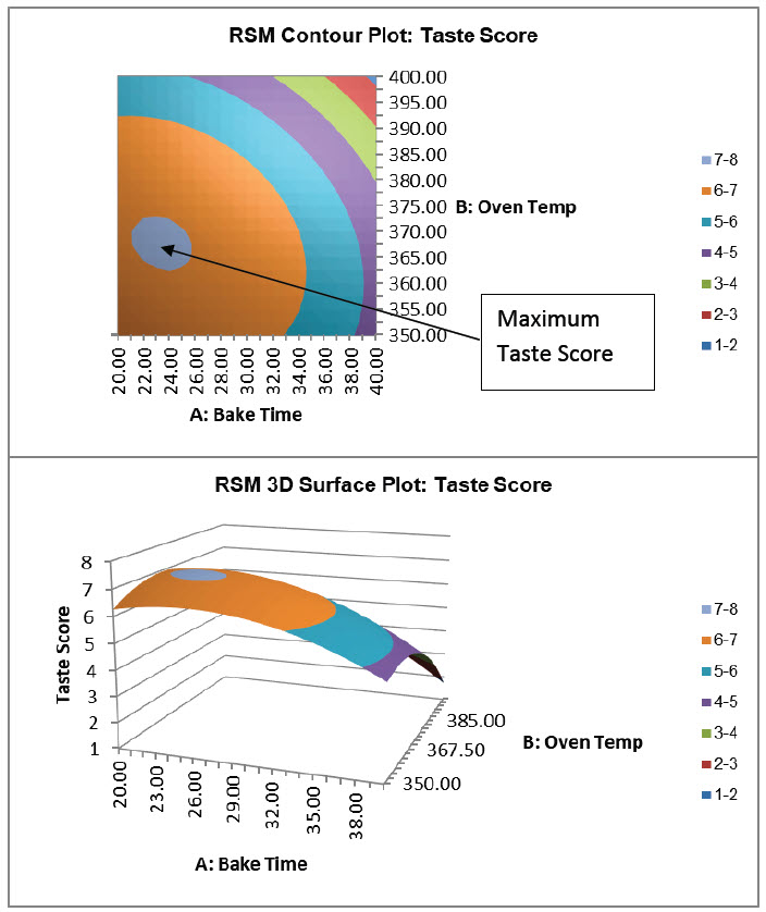
Click OK. The following Contour and Surface Plots are
displayed:
Go to Analyze 2 Factor RSM tab. Scroll across to the
Predicted Response Calculator. Enter the predicted values shown. These
initial settings were determined from the contour plot as an estimate to yield a maximum
taste score.
Note: The RSM Regression Model: Taste
Score equation given above uses the coded coefficients,
so if this equation is used to do predictions, the inputs must
first be coded as done in the Predicted Response Calculator.
Excels Solver may also be used to get a more exact solution:
Although the model is predicting values that exceed the maximum taste score of 7, this
is expected to give us the best possible settings for cook time and bake temperature. To
quote the eminent statistician George Box, All models are wrong, some are useful.
Additional experimental runs carried out at Time = 23.4 minutes and Temperature = 367.7
F. confirm that these are ideal settings.
Analysis of Response Surface Experiment Cake Bake with Advanced Multiple Regression
Open the file RSM Example Cake Bake Data for Adv MReg.xlsx.
This is the RSM Example - Cake Bake data copied into a workbook with
A: and B: removed from the Factor Names as they are not needed for Advanced Multiple Regression.
Click Sheet 1 tab. Click SigmaXL > Statistical Tools > Advanced Multiple Regression > Fit Multiple Regression Model.
If necessary, click Use Entire Data Table, click Next.
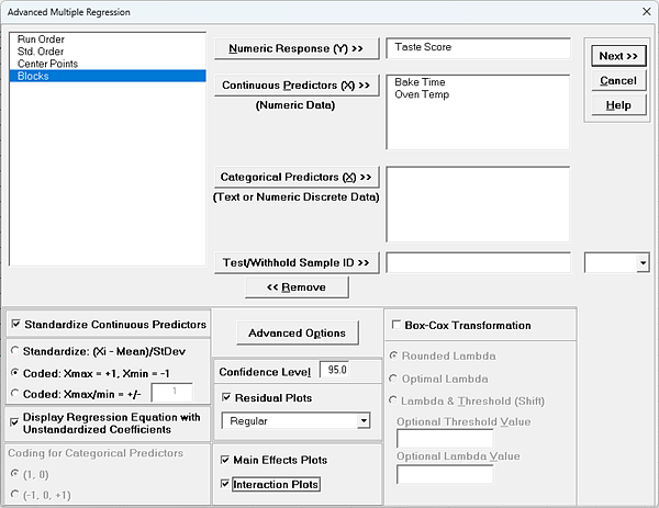
Select Taste Score, click Numeric Response (Y) >>; select Bake Time and Oven Temp; click Continuous Predictors (X) >>.
Check Standardize Continuous Predictors with option Coded:
Xmax = +1, Xmin = -1.
Check Display Regression Equation with Unstandardized Coefficients.
Use the default Confidence Level = 95.0%. Regular Residual Plots are checked by default.
Check Main Effects Plots and Interaction Plots.
Leave Box-Cox Transformation unchecked.
Standardize Continuous Predictors with Coded:
Xmax = +1, Xmin = -1 scales the continuous predictors so that
Xmax is set to +1 and Xmin is set to -1.
This is particularly useful for analyzing data from a 3-Level Face-Centered RSM design of experiments with Alpha axial = 1.0.
If the design was a 5-Level Rotatable with Alpha axial = 1.414, we would have selected Standardize Continuous Predictors with Coded:
Xmax/Xmin = +/- 1.414.
Display Regression Equation with Unstandardized Coefficients displays the prediction equation with unstandardized/uncoded coefficients but the Parameter Estimates table will still show the standardized coefficients. This format is easier to interpret since there is only one coefficient value for each predictor.
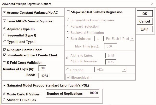
Click Advanced Options. We will use the defaults as shown. Ensure that Stepwise/Best Subsets Regression is unchecked.
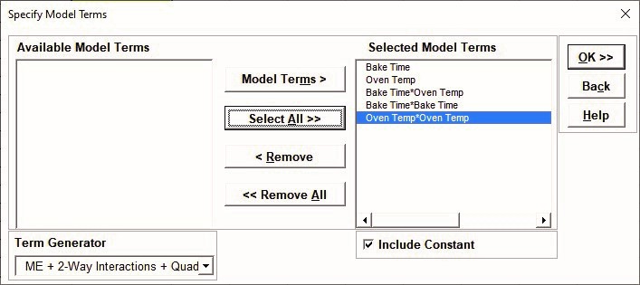
Click OK. Using Term Generator, select ME + 2-Way Interactions + Quadratic. Click Select All >>.
Include Constant is checked by default.
This matches the final model used in the original analysis for Taste Score.
Click OK. The Advanced Multiple Regression report for Taste Score is given:
Note, the prediction equation is uncoded so the coefficients do not match the coded coefficients given in the Parameter Estimates table.
If consistency is desired, one can always rerun the analysis with Display Regression Equation with Unstandardized Coefficients unchecked.
Blanks and special characters in the predictor names of the equation are converted to the underscore character _.
The model summary statistics match the previous analysis.
R-Square Predicted = 97.89%, also known as Leave-One-Out Cross-Validation, indicates how well a regression model predicts responses for new observations and is typically less than R-Square Adjusted.
This is also very good.
The Parameter Estimates and ANOVA match the previous analysis.
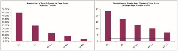
The Pareto Chart of Standardized Effects for Taste Score is similar to the Pareto Chart of Abs(Coefficient) but is based on the term T statistic.
Since this is an orthogonal design, Adjusted (Type III) Sum-of-Squares are the same as Sequential (Type I) Sum-of-Squares (not shown), so the Term R-Square Pareto shows the percent contribution to variability in the Taste Score and sums to R-Square = 98.87%.
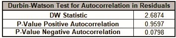
The Durbin-Watson Test for Autocorrelation in Residuals table is:
The Durbin Watson (DW) test is used to detect the presence of positive or negative autocorrelation in the residuals at Lag 1.
If either P-Value is < .05, then there is significant autocorrelation.
Here, there is no significant autocorrelation in the residuals, which is what we would expect in a randomized design of experiments.
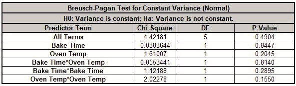
The Breusch-Pagan Test for Constant Variance is:
There are two versions of the Breusch-Pagan (BP) test for Constant Variance: Normal and Koenker Studentized Robust.
SigmaXL applies an Anderson-Darling Normality test to the residuals in order to automatically select which version to use.
If the AD P-Value < 0.05, Koenker Studentized Robust is used.
The report includes the test for All Terms and for individual predictors.
All Terms denotes that all terms are in the model.
This should be used to decide whether or not to take corrective action.
The individual predictor terms are evaluated one-at-a-time and provide supplementary information for diagnostic purposes.
Note, this should always be used in conjunction with an examination of the residual plots.
Here we see that the All Terms test is not significant, so we conclude that the variance is constant.
Tip: If the All Terms test is significant after model refinement, try a Box-Cox transformation.
If that does not work, refit the model using Recall Last Dialog, click Advanced Options in the Advanced Multiple Regression dialog, and uncheck Assume Constant Variance/No AC.
SigmaXL will apply the White robust standard errors for non-constant variance. For details, see the Appendix: Advanced Multiple Regression.
Tip: Lack of Constant Variance (a.k.a. Heteroskedasticity) is a nuisance for regression modelling but is also an opportunity.
Examining the residual plots and individual predictors may yield process knowledge that identifies variance reduction opportunities.
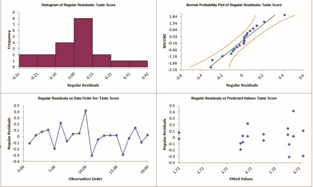
Click on Sheet MReg1 Residuals to view the Residual Plots. Note, Sheet MReg# will increment every time a model is refitted.
The residuals are approximately normal.
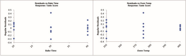
There is a possible pattern in the Residuals vs Oven Temp with Oven Temp = 400 showing less variance, but the Breusch-Pagan test for constant variance for Oven Temp is not significant, so here we cannot conclude that a higher Oven Temp would result in a lower Taste Score variance.
Note: Residuals versus interaction or quadratic terms are not plotted, but they can be manually created using the model design matrix to the right of the Residual Plots (use
SigmaXL > Graphical Tools >
Scatter Plots).
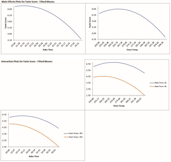
Click on Sheet MReg1 Plots. The Main Effects Plots and Interaction Plots for Taste Score are shown.
These are based on Fitted Means as predicted by the model, not Data Means as used in the previous analysis.
Main Effects Plots with Fitted Means use the predicted value for the response versus input predictor value, while holding all other variables at their respective means.
Similarly for Interaction Plots, all predictors not being plotted are held at their respective means.
The curvature is due to the quadratic terms in the model.
These plots give us an initial look at the Fitted Means for Taste Score, but Contour and Surface Plots will be more useful for this Response Surface Design.
Click on Sheet MReg1 Model. Scroll to the Predicted Response Calculator.
Enter Bake Time = 23, Oven Temp = 368 to predict Taste Score with the 95% confidence interval for the long term mean and 95% prediction interval for individual values:
Note the formula at cell L14 is an Excel formula. This matches the previous initial settings.
Here the full predictor names are used making it easier to use and interpret.
The Coded Settings are calculated as part of the Excel formula. Also, the prediction standard error SE is given.
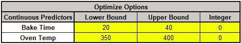
Next, we will use SigmaXLs built in Optimizer. Scroll to view the Optimize Options:
Here we can constrain the lower and upper bounds of the continuous predictors, but we will leave the default settings as is, which are obtained from the minimum and maximum of the predictor values.
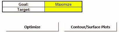
Scroll back to view the Goal setting and Optimize button. Specify Goal = Maximize.
The optimizer uses Multistart Nelder-Mead Simplex to solve for the desired response goal with given constraints.
For more information see the Appendix: Single Response Optimization.
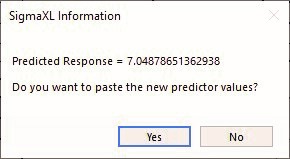
Click Optimize. The response solution and prompt to paste values into the Input Settings of the Predicted Response Calculator is given:
Click Yes to paste the values.
This matches the solution that was obtained using Solver in the previous analysis.
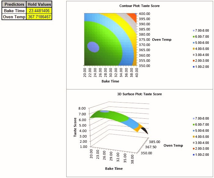
Next, we will create a Contour/Surface Plot. Click the Contour/Surface Plots button.
A new sheet is created, MReg1 Contour that displays the plots:
This matches the Contour and Surface Plots given in the previous analysis.
The table with the Hold Values, gives the values used to hold a predictor constant if it is not in the plot, so is not applicable here with only one plot based on the two continuous predictors.
Tip: Use the contour/surface plots in conjunction with the predicted response calculator to determine optimal settings.