ARIMA Control Charts with Predictors

The ARIMA model supports continuous or categorical predictors, similar to multiple regression in SigmaXL.
In order to provide a forecast, additional predictor (X) values must be added to the dataset prior to running the analysis. The number of forecast periods will be equal to the number of additional predictor rows. Alternatively, the predictor values from a withhold sample may be used. If neither are provided, SigmaXL will use the last row of predictor values and compute one forecast period.

Continuous predictors are numeric, categorical predictors can be text or numeric. All predictors must have the same number of rows. A predictor cannot have all values the same.

As with multiple linear regression, predictors should not be strongly correlated. SigmaXL will automatically remove terms with very high variance inflation factors (VIF > 100) and give a warning message “Multicollinearity detected in predictors. The following predictors were removed…”.

Also as done in multiple linear regression, categorical predictors are automatically “dummy coded”. Predictors will have a level append to their term names in the Parameter Estimates table. The first level (sorted alphanumerically) is a hidden reference level. If there are three levels, only two will appear in the Parameter Estimates table.

Missing values, while permitted in the Time Series Data (Y), are not permitted in the predictors. A warning message will be given, “Missing values detected in predictors. The following predictors were removed…”. If all predictors have missing values an error message is returned. An exception is made for missing values in the first rows to accommodate indicators with lags.

Sometimes the impact of a predictor will not be simple and immediate. For example, an advertising campaign may impact sales for some time beyond the end of the campaign, and sales in one month will depend on the advertising expenditure in each of the past few months. In these situations, we need to allow for lagged effects of the predictor (Hyndman, fpp2, 9.6 Lagged Predictors). A Pre-Whitened CCF Plot will show which lags need to be included in the model. SigmaXL can accommodate lagged predictors, but they must be manually created using SigmaXL > Utilities > Lag Data (or simply: copy, shift down one row, paste new column, delete extra row at bottom, add column header for the predictor data, and include as a predictor in the ARIMA model). Note, Box and Jenkins, Ch. 11, describe a more complex model method called a Transfer Function, but this is not provided in SigmaXL.

Open Daily Electricity Demand with Predictors – ElecDaily.xlsx (Sheet 1 tab). This is daily electricity demand (GW) for the state of Victoria, Australia, every day during 2014. Temp (C) is the maximum daily temperature in degrees Celsius for the city of Melbourne. TempSq is Temperature squared. WorkDay takes on the value 1 on work days and 0 otherwise. This data has a seasonal frequency = 7 (observations per week). See the Run Chart, ACF/PACF Plots, Spectral Density Plot and Seasonal Trend Decomposition Plots for this data.

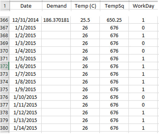
Click the Forecast 2 Weeks Sheet tab. Following the referenced example, we will use the ARIMA model to forecast 14 days ahead starting from January 1, 2015 (a non-work-day being a public holiday for New Year’s Day). We could obtain weather forecasts for those 14 days, but for the sake of illustration, we will set the temperature for the 14 days to a constant 26 degrees and TempSq to 676. Scroll down to view the added data. Note that Date, Temp (C), TempSq and WorkDay are added for these 14 days, but the Demand values are blank:

Click SigmaXL > Time Series Forecasting > ARIMA Forecast > Forecast with Predictors. Ensure that the entire data table is selected. If not, check Use Entire Data Table. Click Next.

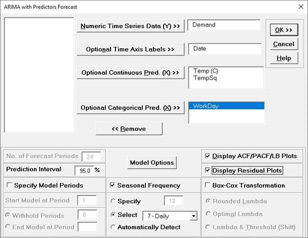
Select Demand, click Numeric Time Series Data (Y) >>; select Date, click Optional X-Axis Labels >>; select Temp (C) and TempSq, click Optional Continuous Pred. >>; select WorkDay, click Optional Categorical Pred. >>. Check Display ACF/PACF/LB Plots and Display Residual Plots. Check Seasonal Frequency with Select = 7 - Daily (or Specify = 7). Leave Specify Model Periods and Box-Cox Transformation unchecked. We will use the default Prediction Interval = 95.0 %.
- No. of Forecast Periods is greyed out because they are determined by the number of additional predictor rows that are provided, in this example, 14.
- Optional Continuous Pred. (X) are continuous predictors.
- Optional Categorical Pred. (X) are categorical predictors. In this example WorkDay could be either continuous or categorical since it is coded as 0,1.

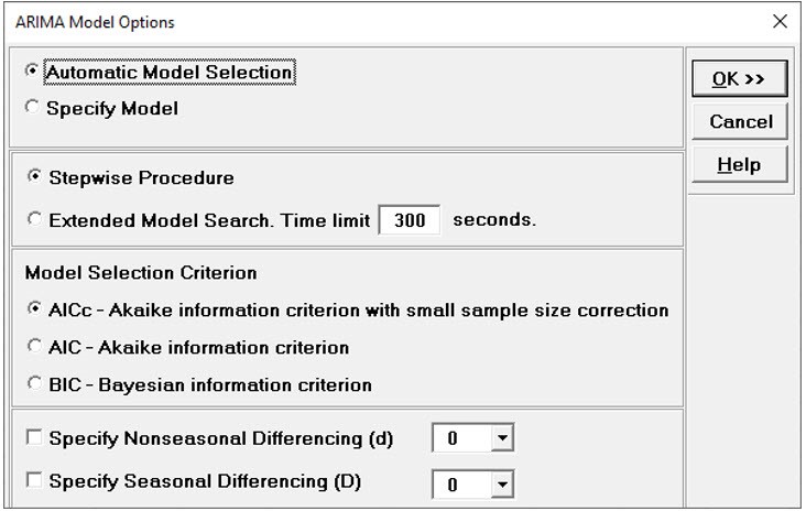
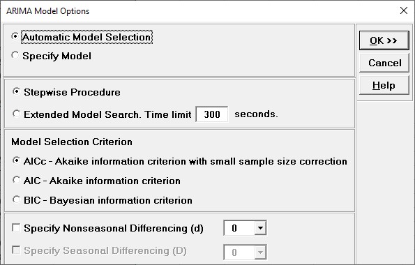
Click Model Options. Select Automatic Model Selection. We will use the defaults: Stepwise Procedure and Model Selection Criterion: AICc – Akaike information criterion with small sample size correction, leave Specify Nonseasonal Differencing (d) and Specify Seasonal Differencing (D) unchecked.

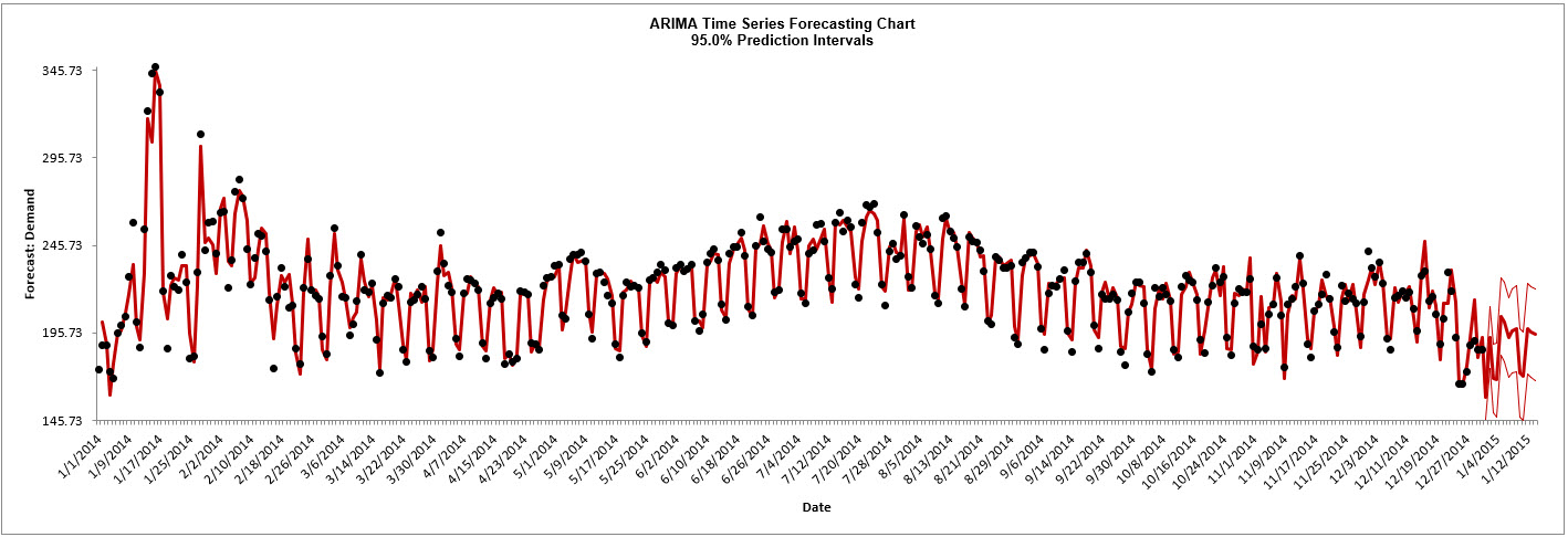
Click OK to return to the ARIMA Forecast dialog. Click OK. This is a complex model, so computation time will be approximately one to two minutes. The ARIMA forecast report is given:

This agrees with Figure 9.8 given in Hyndman, fpp2, Section 9.3, Example: Forecasting electricity demand, https://otexts.com/fpp2/forecasting.html. There are slight differences in the initial predicted values.

Scroll down to view the ARIMA Model header:

If we had checked Specify Model Periods in the main dialog, the start, end or withhold selection would be summarized here as well.

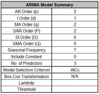
The ARIMA Model Summary is given as:

This is a summary of the model information: ARIMA (2,1,2) (2,0,0) with no constant and 3 predictors. Seasonal Frequency = 7; Model Selection Criterion = “AICc” and Box-Cox Transformation = “N/A” because Box-Cox Transformation was unchecked.

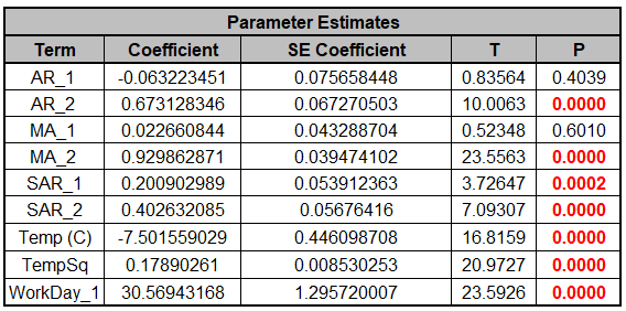
The Parameter Estimates are:

ARIMA Parameter Estimates include significance tests; P-Values < .05 are significant and highlighted in red. All of the predictors are significant. The AR_1 and MA_1 terms are not significant but they must remain in the model due to hierarchy. Note that for AR/MA model order selection, minimum AICc should be used, rather than significance tests (see Kostenko, A.V. and Hyndman, R.J.).

The categorical predictor WorkDay_1 has 0 as the hidden reference level. If there were three category levels, only two would appear in the table.

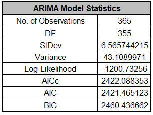
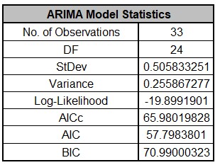
The ARIMA Model Statistics are:

Degrees of freedom (DF) = n – 10 (9 terms in the model, 1 order of differencing).

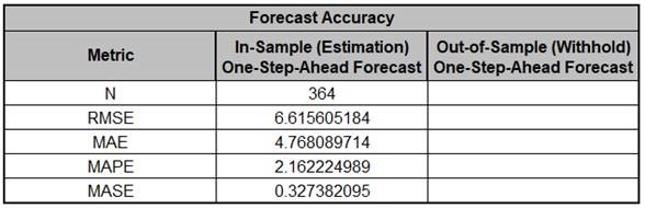
The In-Sample Forecast Accuracy metrics are:

MASE is less than one, so it is a better forecast than would be obtained from a naïve forecast (set all forecasts to be the value of the last observation).

The analysis can be rerun (using Recall SigmaXL Dialog) with a withhold sample to obtain Out-of-Sample One-Step-Ahead or Multi-Step-Ahead Forecast errors, but we will not do so here.

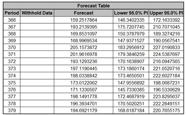
The Forecast Table is given as:

These are the same forecast and prediction interval values displayed in the Forecast Chart but provided for further analysis or charting. If Withhold Periods are specified, the Withhold Data will be displayed as well.

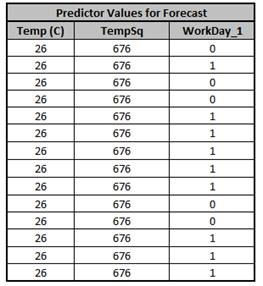
The Predictor Values for Forecast are the additional predictor (X) values used to obtain the 14 period forecast in the Forecast Table:

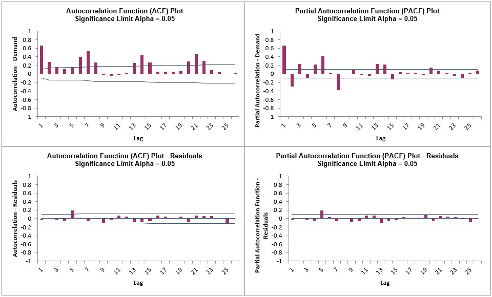
Click on the ARIMA ACF PACF LB sheet to view the ACF/PACF/LB Plots:

We can see that much of the autocorrelation has been removed by the ARIMA with Predictors model (with the exception of lag 5 and 25 in the ACF, lag 5 in the PACF).

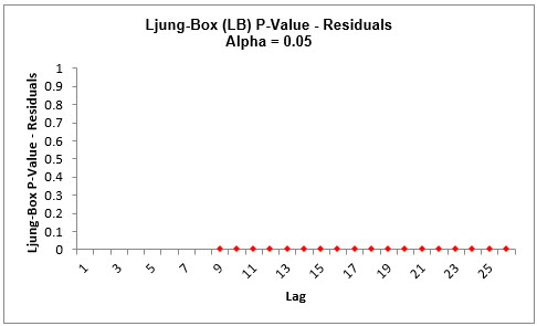
The Ljung-Box plot shows that some significant autocorrelation still remains (the red P-Values are significant at alpha=.05) - so the model can potentially be improved. This does not mean that the model is a bad model, it can still be very useful for prediction purposes, but the prediction intervals may not provide accurate coverage.

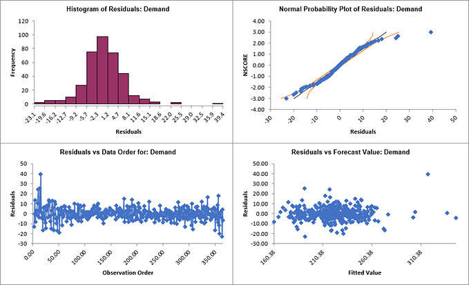
Click on the ARIMA Residuals sheet to view the Residual Plots:

Looking at the histogram and normal probability plot, there are some outliers (but smaller than would have been the case if we did not include the predictors). Later, these will be investigated with a control chart on the residuals.

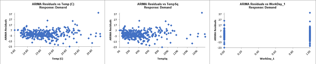
Note that additional residual plots are provided for each predictor.

Open Sales with Indicator - Modified Series M.xlsx. This is modified Series M data from Box and Jenkins. Originally, a set of 150 monthly corporate sales values along with a leading indicator, the data was modified by converting it to quarterly values by averaging every three months, so 50 quarters, labelled as Q1-Y1, Q2-Y1, etc. This was done in order to simplify the analysis of the leading indicator. Although the data was monthly and summarized to quarterly, it will be treated as nonseasonal, as done in Box and Jenkins. See the Run Chart, ACF/PACF Plots, CCF Plot, Spectral Density Plot and Trend Decomposition Plots for this data.

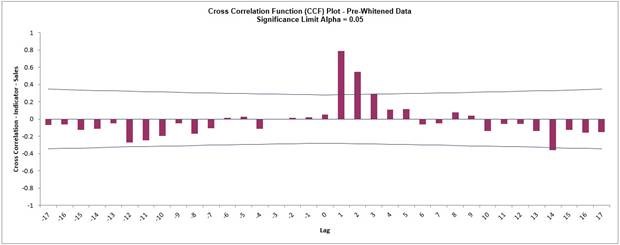
Recall that the Pre-Whitened CCF Plot for this data is:

Pre-Whitening the data has dramatically altered the CCF plot, allowing us to see the underlying cross correlation pattern. Lags 1 and 2 are significantly positive, and Lag 3 is just on the significance line. Use this as a guide to assist with what lags to include in the model but it is possible that some additional lags may be significant. In this example, we will initially include up to Lag 5.

Note that while X is called a leading indicator, i.e., X comes before Y in time, the positive lag means that the X variable is lagging the Y variable in terms of correlation structure. SigmaXL uses this convention as given in Box and Jenkins (2016, pp. 437-440).

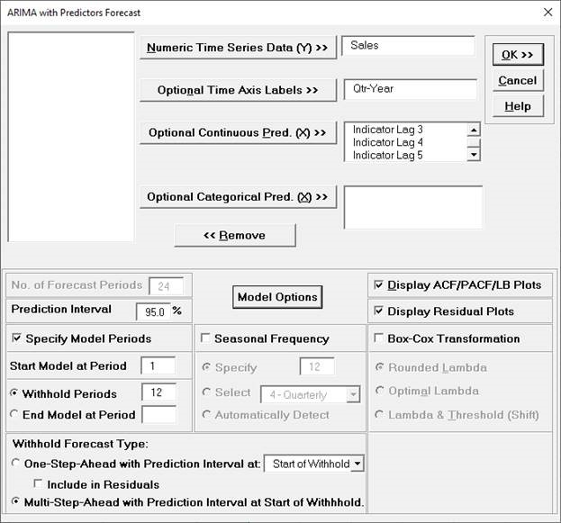
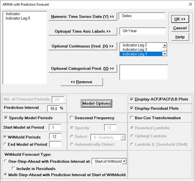
Click the Indicator with Lags Sheet tab. SigmaXL > Time Series Forecasting > ARIMA Forecast > Forecast with Predictors. Ensure that the entire data table is selected. If not, check Use Entire Data Table. Click Next.

Select Sales, click Numeric Time Series Data (Y) >>; select Qtr-Year, click Optional Time Axis Labels >>; select Indicator to Indicator Lag 5, click Optional Continuous Pred. >>. Check Display ACF/PACF/LB Plots and Display Residual Plots. Check Specify Model Periods. Set Withhold Periods = 12 (i.e., 3 years). Select Withhold Forecast Type: Multi-Step-Ahead with Prediction Interval at Start of Withhold. Leave Specify Model Periods, Seasonal Frequency and Box-Cox Transformation unchecked. We will use the default Prediction Interval = 95.0 %.

Click Model Options. Select Automatic Model Selection. We will use the defaults: Stepwise Procedure and Model Selection Criterion: AICc – Akaike information criterion with small sample size correction, leave Specify Nonseasonal Differencing (d) and Specify Seasonal Differencing (D) unchecked.

Tip: When using Recall SigmaXL Dialog and if there are no changes to the Model Option settings, the previous settings will be used. It is not necessary to repeat this step.

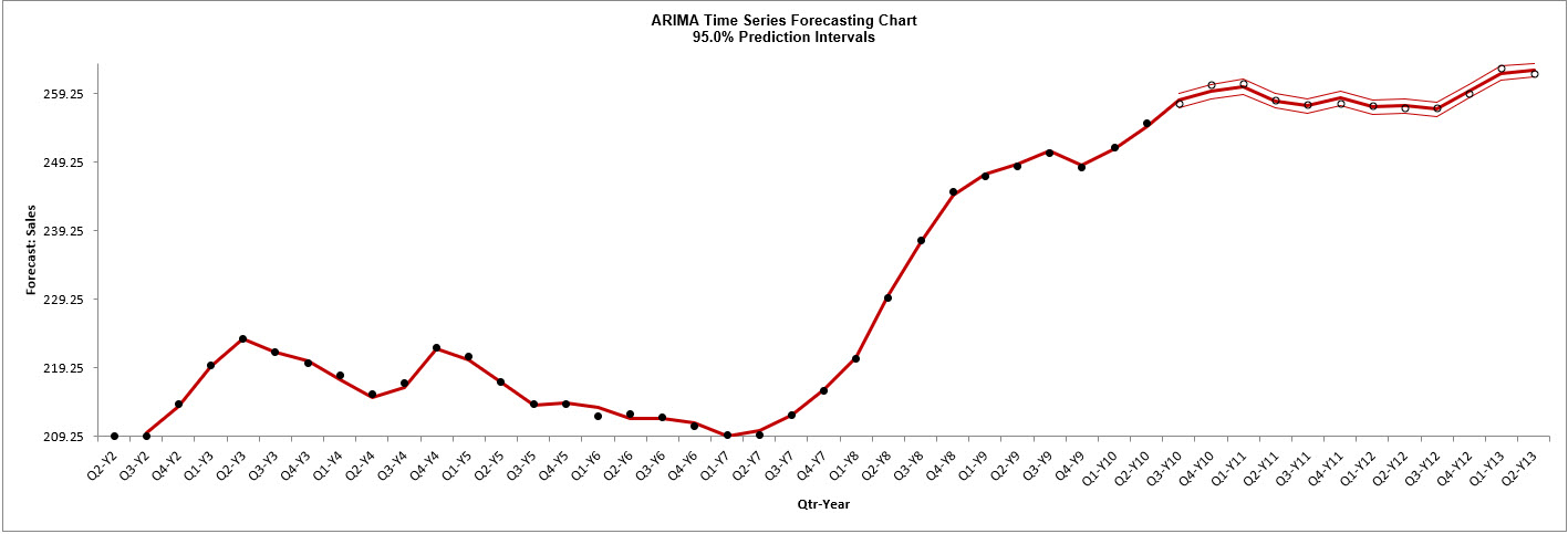
Click OK to return to the ARIMA Forecast dialog. Click OK. The ARIMA with Predictors forecast report is given:

The blank dots are the data values in the withhold sample with a multi-step forecast and prediction intervals displayed at the start of the withhold sample. The model uses the Indicator Lag values in the withhold sample and does quite well at predicting the 12 quarters of Sales values.

Note that the chart starts at Q2-Y2. This is due to the first 5 rows of X and Y data being deleted since there are missing values in Indicator Lags 1 to 5.

Scroll down to view the ARIMA Model header:

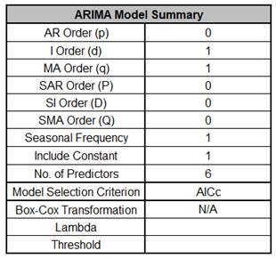
The ARIMA Model Summary is given as:

This is a summary of the model information: ARIMA (0,1,1) with no constant and 6 predictors. Seasonal Frequency = 1 (nonseasonal); Model Selection Criterion = “AICc” and Box-Cox Transformation = “N/A” because Box-Cox Transformation was unchecked.

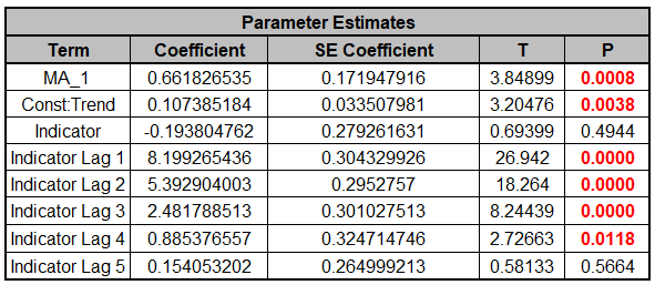
The Parameter Estimates are:

ARIMA Parameter Estimates include significance tests; P-Values < .05 are significant and highlighted in red. The CCF Plot suggested that only Lags 1 and 2, possibly 3, would be significant, but here we see that Lag 4 is also significant (hence why CCF is just an approximate guide). Later we will rerun the model and remove Indicator & Indicator Lag 5 and manually compare AICc values.

The ARIMA with Predictors Model Statistics are:
- The number of observations, n = 50 – 12 (withhold) – 5 (deleted rows) = 33
- Degrees of freedom (DF) = 33 (n) – 9 (8 terms in the model, 1 nonseasonal difference) = 24
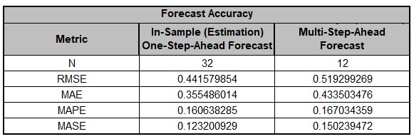
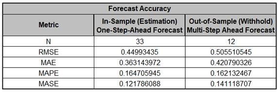
The Forecast Accuracy metrics are:

The Out-of-Sample forecast errors are only slightly larger than the In-Sample, so this is a good prediction.

MASE is less than one, so it is a better forecast than would be obtained from a naïve forecast (set all forecasts to be the value of the last observation).

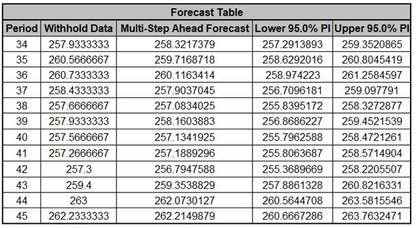
The Forecast Table is given as:

These are the same forecast and prediction interval values displayed in the Forecast Chart but provided for further analysis or charting. Note that this table gives the Forecast Period number whereas the Chart displays the Quarter-Year.

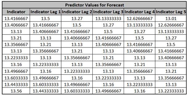
The Predictor Values for Forecast are the additional predictor (X) values used to obtain the 12 period forecast in the Forecast Table:

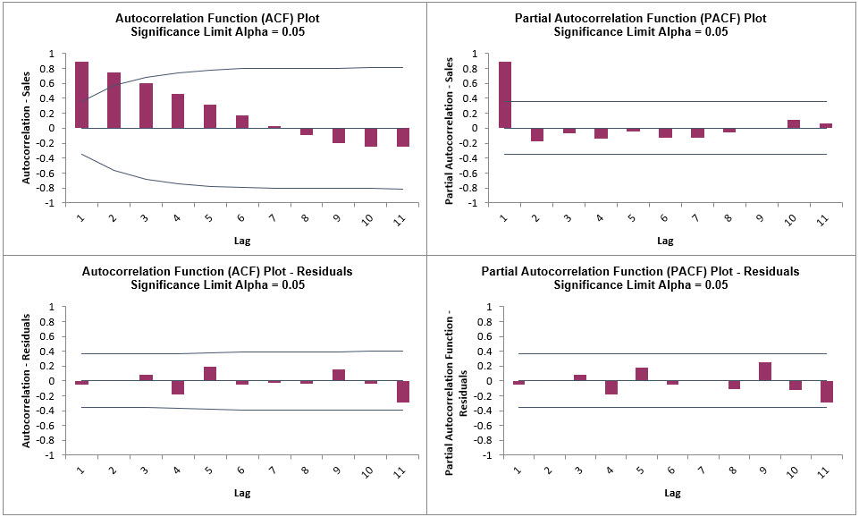
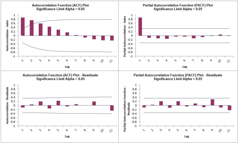
Click on the ARIMA ACF PACF LB sheet to view the ACF/PACF/LB Plots:

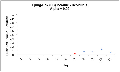
We can see that much of the autocorrelation has been removed by the ARIMA with Predictors model. The Ljung-Box plot shows that some significant autocorrelation still remains (the red P-Values are significant at alpha = .05) - so the model can potentially be improved. This does not mean that the model is a bad model, it can still be very useful for prediction purposes, but the prediction intervals may not provide accurate coverage.

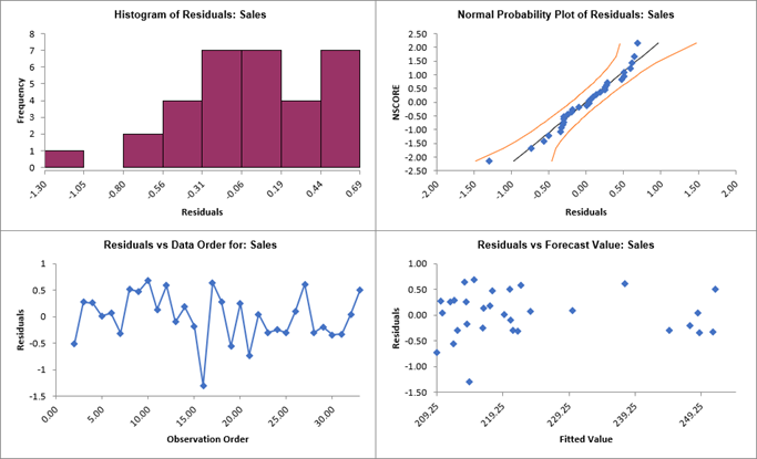
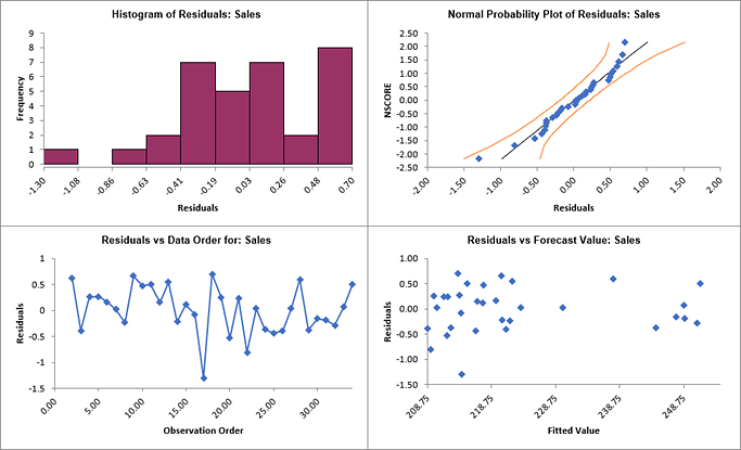
Click on the ARIMA Residuals sheet to view the Residual Plots:

The residuals are approximately normally distributed, with a roughly straight line on the normal probability plot. There are no obvious extreme outliers or patterns in the charts. The histogram might suggest a left skew but the sample size is quite small. (Normality tests may also be applied on the residuals using SigmaXL > Statistical Tools > Descriptive Statistics: Options, Additional Normality Tests, and these would all show the residuals to be normal).

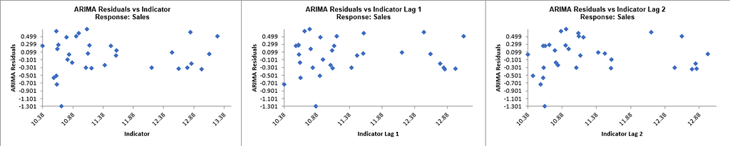
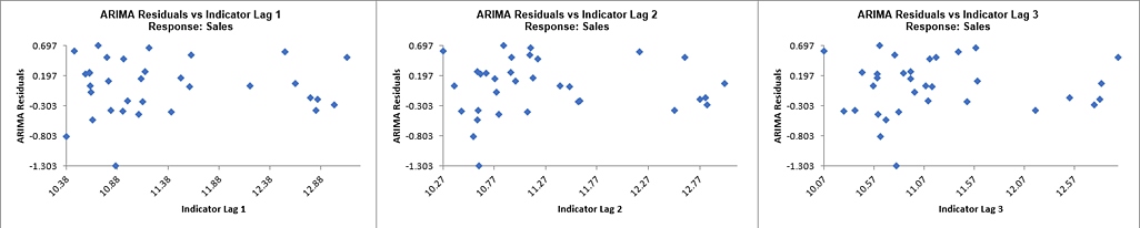
Note that additional residual plots are provided for each predictor.

Now we will rerun the analysis and remove the insignificant terms Indicator and Indicator Lag 5. Click Recall SigmaXL Dialog menu or press F3 to recall last dialog.

Select Indicator, click Remove; select Indicator Lag 5, click Remove:

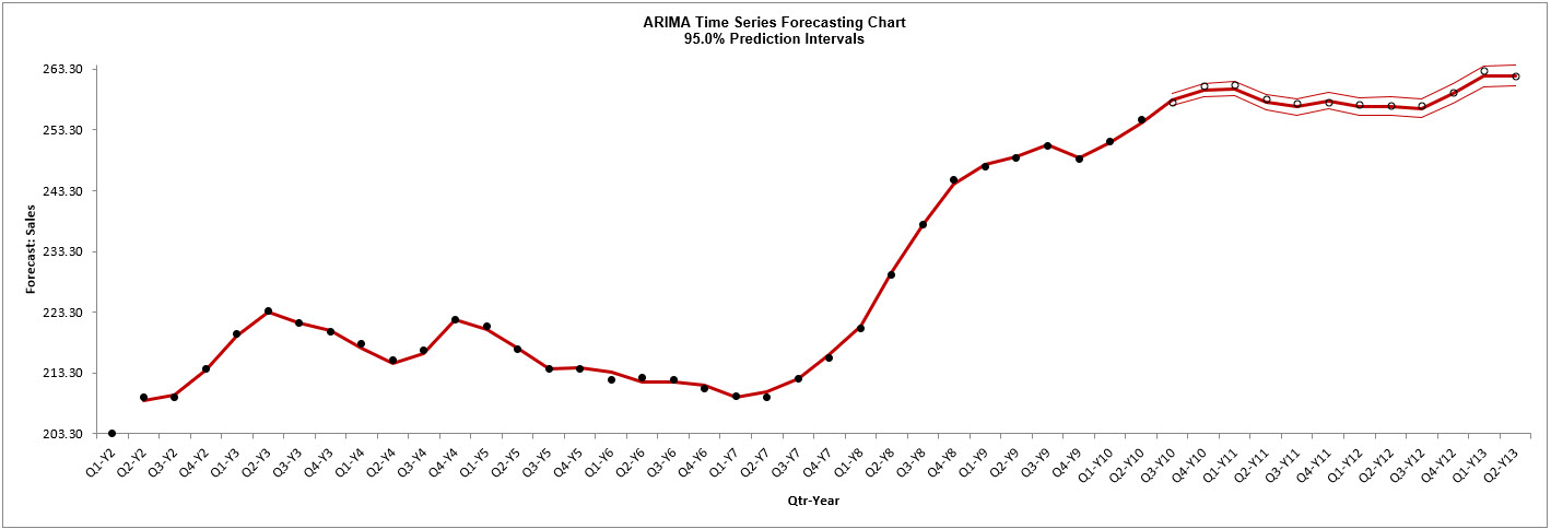
We will not make any changes to the Model Options. Click OK. The revised ARIMA with Predictors forecast report is given:

Note that the chart now starts at Q1-Y2. This is due to the first 4 rows of X and Y data being deleted since there are missing values in Indicator Lags 1 to 4.

Scroll down to view the ARIMA Model header:

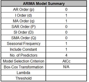
The ARIMA Model Summary is given as:

This is a summary of the model information: ARIMA (0,1,1) without a constant has not changed. Now there are 4 predictors. Seasonal Frequency = 1 (nonseasonal); Model Selection Criterion = “AICc” and Box-Cox Transformation = “N/A” because Box-Cox Transformation was unchecked.

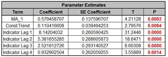
The Parameter Estimates are:

ARIMA Parameter Estimates include significance tests; P-Values < .05 are significant and highlighted in red. The CCF Plot suggested that only Lags 1 and 2, possibly 3, would be significant, but here we see that Lag 4 is also significant (hence why CCF is just an approximate guide).

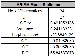
The ARIMA with Predictors Model Statistics are:
- The number of observations, n = 50 – 12 (withhold) – 4 (deleted rows) = 34
- Degrees of freedom (DF) = 34 (n) – 7 (6 terms in the model, 1 nonseasonal difference) = 27
- AICc is lower than the previous model which included insignificant Indicator terms.

The Forecast Accuracy metrics are:

Compared to the previous Forecast Accuracy metrics the Out-of-Sample forecast errors are slightly lower, so this is a good prediction with a simpler model. MASE is less than one, so it is a better forecast than would be obtained from a naïve forecast (set all forecasts to be the value of the last observation).

Click on the ARIMA ACF PACF LB sheet to view the ACF/PACF/LB Plots:

We can see that much of the autocorrelation has been removed by the ARIMA with Predictors model. The Ljung-Box plot shows fewer significant P-Values than the previous model.

Click on the ARIMA Residuals sheet to view the Residual Plots:

The residuals look similar to those in the previous model, approximately normally distributed, with a roughly straight line on the normal probability plot. There are no obvious extreme outliers or patterns in the charts. The histogram might suggest a left skew but the sample size is quite small. (Normality tests may also be applied on the residuals using SigmaXL > Statistical Tools > Descriptive Statistics: Options, Additional Normality Tests, and these would all show the residuals to be normal).

Note that additional residual plots are provided for each predictor, Indicator Lag 1 to 4.