ARIMA Control Chart

Open Chemical Process Concentration – Series A.xlsx (Sheet 1 tab). This is the Series A data from Box and Jenkins, a set of 197 concentration values from a chemical process taken at two-hour intervals. See the Run Chart, ACF/PACF Plots, Spectral Density Plot and Seasonal Trend Decomposition Plots for this data.
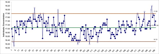
Earlier we saw that this process has significant autocorrelation. In order to see the impact on a control chart, we will construct an Individuals chart on the raw data. Click SigmaXL > Control Charts > Individuals. Ensure that the entire data table is selected. If not, check Use Entire Data Table. Click Next.
Select Concentration, click Numeric Data Variable (Y) >>. Click OK. An Individuals Control Chart is produced:

There are 17 out-of-control data points, largely due to the autocorrelation. Searching for assignable causes using this chart as is, would be futile.
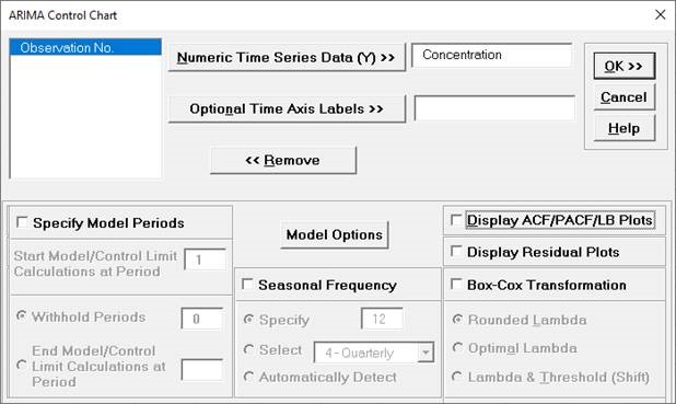
Now click Sheet 1 tab and SigmaXL > Time Series Forecasting > ARIMA Control Chart > Control Chart. Ensure that the entire data table is selected. If not, check Use Entire Data Table. Click Next.
Select Concentration, click Numeric Time Series Data (Y) >>. Uncheck Display ACF/PACF/LB Plots. Leave Display Residual Plots, Specify Model Periods, Seasonal Frequency and Box-Cox Transformation unchecked.
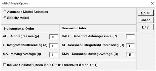
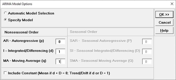
Click Model Options. Select Specify Model. Specify Nonseasonal Order I – Integrated/Differencing (d) = 1 and MA – Moving Average (q) = 1. Leave Include Constant unchecked.

Typically, one would use Automatic Model Selection, but we want to demonstrate the ARIMA control chart using the ARIMA (0,1,1) model as used above, and to compare to the equivalent Exponential Smoothing Control Charts.
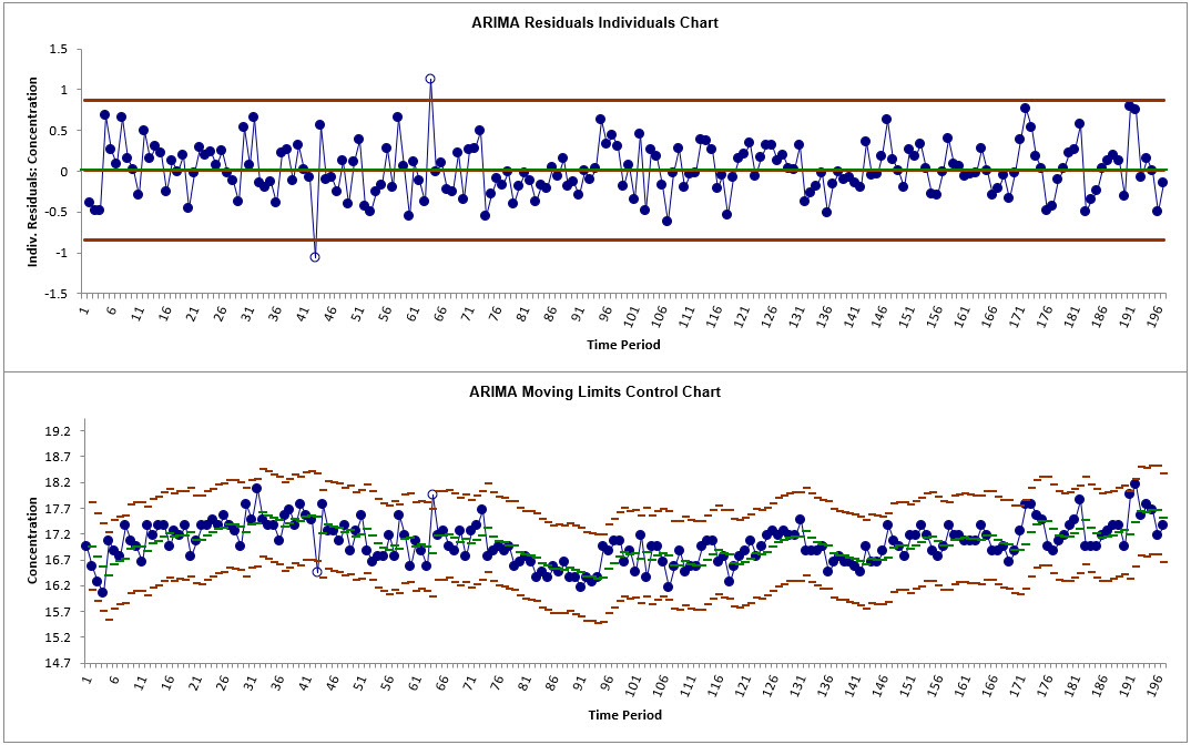
Click OK to return to the ARIMA Control Chart dialog. Click OK. The ARIMA control charts are produced:

Now we only have two out-of-control data points on the Individuals chart to investigate. The Moving Limits chart uses the one step prediction as the center line, so the control limits move with the center line.

As expected, these are approximately the same as the Exponential Smoothing Control Charts, with slight differences on the initial values. The ARIMA Residuals Individuals Chart does not show a data point at Time Period = 1 due to the differencing.
We will scroll through the chart data points as done in the Exponential Smoothing Control Charts. Click SigmaXL Chart Tools > Enable Scrolling.

You may be prompted with a warning message that custom formatting on the chart will be cleared. You can avoid seeing this warning by checking Save this choice as default and do not show this form again.
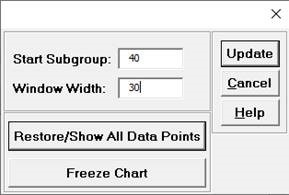
Click OK. The scroll dialog appears allowing you to specify the Start Subgroup and Window Width. Enter Start Subgroup = 40 and Window Width = 30 to view the two out-of-control data points.
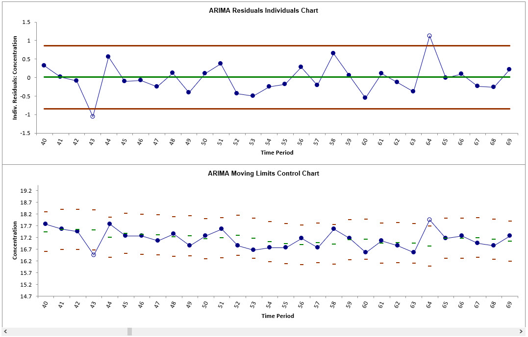
Click OK. This allows us to zoom in on the out-of-control points at 43 and 64.

Observation 43 is lower than expected from the ARIMA forecast model. Observation 64 is higher than expected.
Click Cancel to exit the scroll dialog.
Now we will add a new data point to the Series A Concentration Data. The residuals will be computed using the same model as above without re-estimation of the model parameters or recalculation of the control limits. 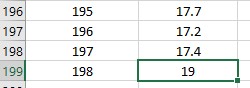This is also known as the “Phase II” application of a Control Chart, where an out-of-control signal should lead to an investigation into the assignable cause and corrective action or process adjustment applied. Click Sheet1, enter the value 19 as shown in cell B199 (and optionally Observation number 198 in cell A199).
Click ARIMA Control Charts tab (if more than one control chart sheet exists in the workbook, please select the chart where the data will be added).
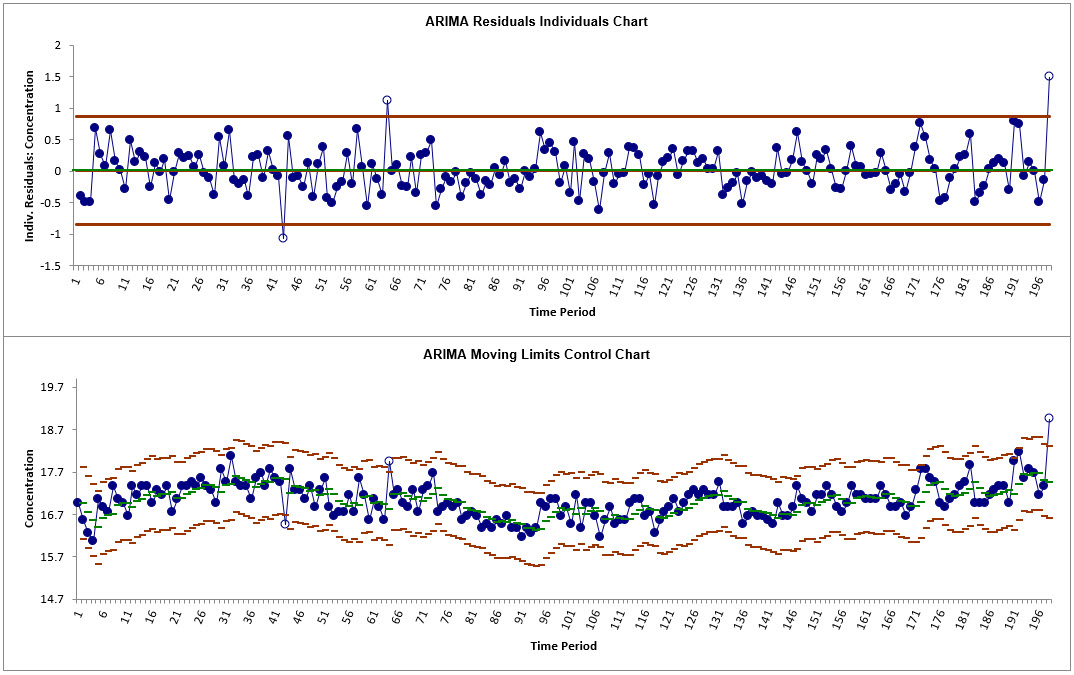
Click SigmaXL Chart Tools > Add Data to this Control Chart
The Residuals Individuals Control Chart and Moving Limits Charts are now updated with the new data, showing this as an out-of-control data point:

We recommend renaming the workbook to Chemical Process Concentration – Series A_AddData2.xlsx, so that later use of the Concentration data does not include the added data point.
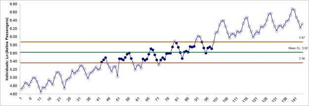
Open Monthly Airline Passengers – Modified for Control Charts.xlsx (Sheet 1 tab). This is based on the Series G data from Box and Jenkins, monthly total international airline passengers for January 1949 to December 1960. A Ln transformation is applied (avoiding the need for a Box-Cox transformation), a negative outlier is added at 50 (-.25) and a level shift applied (+.25), starting at 100. Coded variables were added to help distinguish an outlier versus a shift and they will be analyzed later using ARIMA Forecast with Predictors.
Earlier we saw that this process has significant autocorrelation with a strong trend and seasonality. In order to see the impact on a control chart, we will construct an Individuals chart on the raw data. Click SigmaXL > Control Charts > Individuals. Ensure that the entire data table is selected. If not, check Use Entire Data Table. Click Next.
Select Ln (Airline Passengers), click Numeric Data Variable (Y) >>. Click OK. An Individuals Control Chart is produced:

With strong trend, seasonality and positive autocorrelation, this control chart is meaningless.
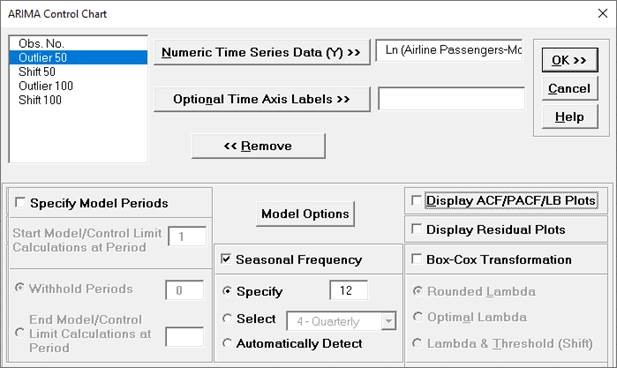
Now click Sheet 1 tab and SigmaXL > Time Series Forecasting > ARIMA Control Chart > Control Chart. Ensure that the entire data table is selected. If not, check Use Entire Data Table. Click Next.
Select Ln(Airline Passengers-Modified), click Numeric Time Series Data (Y) >>. Uncheck Display ACF/PACF/LB Plots and Display Residual Plots. Check Seasonal Frequency with Specify = 12. Leave Specify Model Periods and Box-Cox Transformation unchecked.
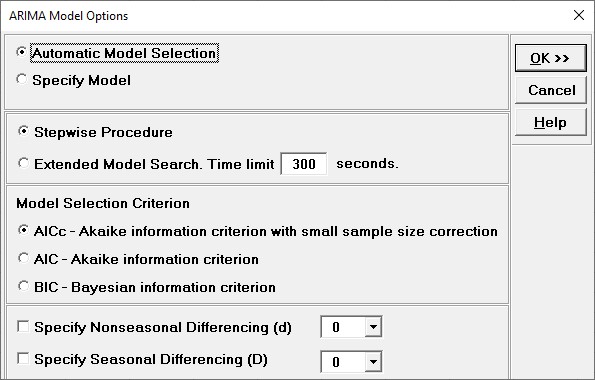
Click Model Options.
We will use the default Automatic Model Selection with AICc as the Model Selection Criterion. Click OK to return to the ARIMA Control Chart dialog. Click OK. The ARIMA control charts are produced:

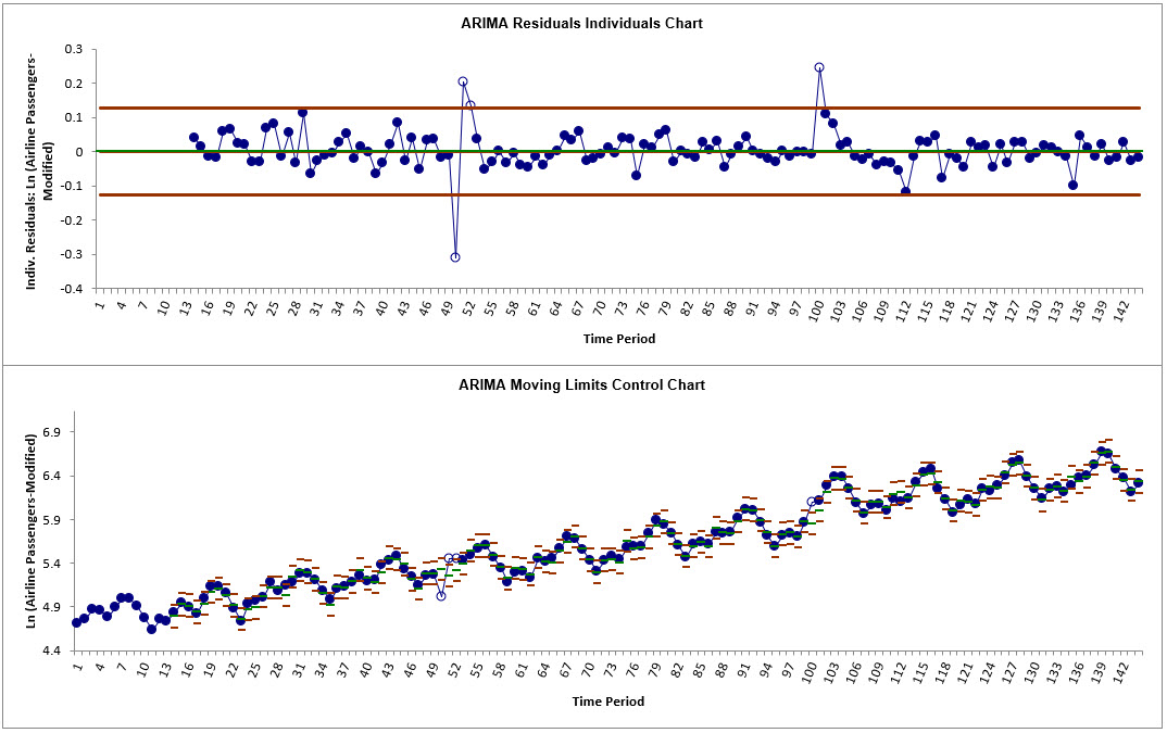
Now we can clearly see the out-of-control data points at 50, 51, 52 and 100 on the Individuals chart. These are approximately the same as those given in Exponential Smoothing Control Charts (52 was in-control). The ARIMA Residuals Individuals Chart does not show data points at Time Periods 1 to 13 due to the nonseasonal and seasonal differencing.
In order to view the points on the Moving Limits chart we will use scrolling. Click SigmaXL Chart Tools > Enable Scrolling

You may be prompted with a warning message that custom formatting on the chart will be cleared. You can avoid seeing this warning by checking Save this choice as default and do not show this form again.
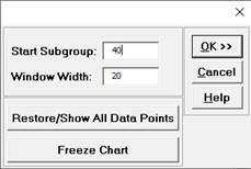
Click OK. The scroll dialog appears allowing you to specify the Start Subgroup and Window Width. Enter Start Subgroup = 40 and Window Width = 20 to view the first two out-of-control data points.
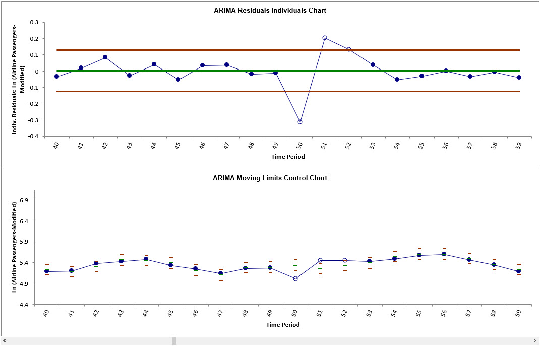
Click OK. This allows us to zoom in on the out-of-control points at 50, 51 and 52.

Observation 50 is lower than expected from the ARIMA forecast model. Observations 51 and 52 are higher than expected.

Tip: Scrolling keeps the original Y axis minimum and maximum setting. You may wish to change this to auto by clicking on the Y axis, right click Format Axis, click Bounds Minimum Reset and Bounds Maximum Reset. This changes the axis settings to Auto so when you scroll or Update the Y axis will automatically adjust as well.
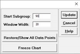
Now enter Start Subgroup = 90 and Window Width = 20 to view the third out-of-control data point.
Click Update.

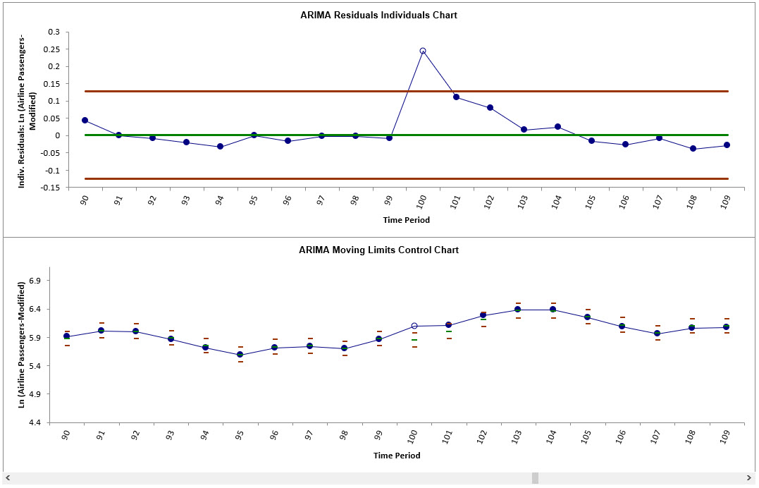
Observation 100 is higher than expected from the ARIMA forecast model. Later investigation will reveal that this is a shift in the mean.
Click Cancel to exit the scroll dialog.
Scroll down to view the ARIMA Model header:
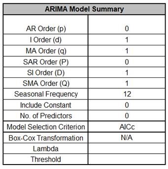
The ARIMA Model Summary is:

The ARIMA (0,1,1) (0,1,1) model (with no constant) was automatically selected based on the AICc criterion. This is the same as we obtained earlier when using a withhold sample and agrees with the results shown in the ACF/PACF Plots of the manually differenced data and is the model used in Box and Jenkins, Chapter 9., “Analysis of Seasonal Time Series”.

There are no predictors. Seasonal Frequency = 12; Model Selection Criterion = “AICc” and Box-Cox Transformation = “N/A”.
The Parameter Estimates and ARIMA Model Statistics are slightly different than our earlier analysis because we have introduced an outlier and a shift, as well here we are using all of the data, i.e., there are no withhold periods. Note that earlier we used a Box-Cox Transformation with Lambda=0 and here we are using Ln of the data.
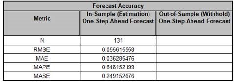
The Forecast Accuracy metrics are given as:

Note that these forecast errors are very different than our earlier analysis, where the forecast errors were calculated on the raw data versus final predicted values, but here we are using Ln of the Airline Passenger data.
Now we will reanalyze the data to determine whether the out-of-control signals are due to an outlier or process shift. Click the Sheet 1 tab.

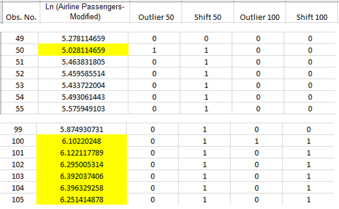
The first out-of-control signal occurred at Obs. No = 50, so two coded variables were created. Outlier50 is coded so that Obs. No. 50 = 1 and all other values are 0. Shift50 is coded so that Obs. No. 1 to 49 = 0, and Obs. No. 50 to 144 are 1.

To simplify the analysis, we will assume that the out-of-control signals at 51 and 52 are related to 50, so will ignore those. The next out-of-control signal occurs at 100, so similarly another two coded variables were created. Outlier100 is coded so that Obs. No. 100 = 1 and all other values are 0. Shift100 is coded so that Obs. No. 1 to 99 = 0, and Obs. No. 100 to 144 are 1.

Since these are coded as 0, 1 we will treat them as Continuous.
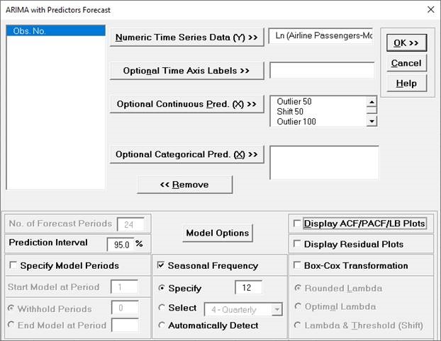
Click SigmaXL > Time Series Forecasting > ARIMA Forecast > Forecast with Predictors. Ensure that the entire data table is selected. If not, check Use Entire Data Table. Click Next.
Select Ln(Airline Passengers – Modified), click Numeric Time Series Data (Y) >>; select Outlier50 to Shift100, click Optional Continuous Pred. >> (. Uncheck Display ACF/PACF/LB Plots and Display Residual Plots. Check Seasonal Frequency with Specify = 12. Leave Specify Model Periods and Box-Cox Transformation unchecked. We will use the default Prediction Interval = 95.0 %.
Click Model Options. With the addition of the coded predictors, we want to ensure that the ARIMA model is the same as that used in the control chart. Select Specify Model. Specify Nonseasonal Order I – Integrated/Differencing (d) = 1 and MA – Moving Average (q) = 1. Specify Seasonal Order SI – Seasonal Integrated/Differencing (D) = 1 and SMA – Seasonal Moving Average (Q) = 1. Leave Include Constant unchecked.
Click OK to return to the ARIMA Forecast dialog. Click OK. The ARIMA forecast report is given.
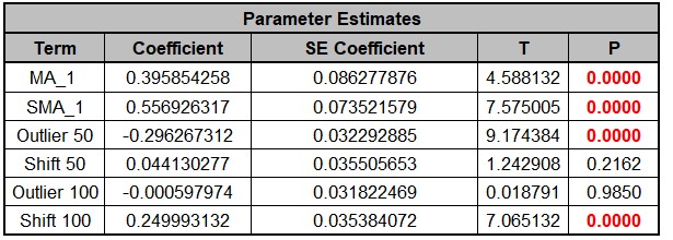
Scroll down to view the Parameter Estimates.

Now we can see that Outlier50 and Shift100 are significant denoting Obs. No. 50 as an outlier and 100 as a shift. This is, of course, what we expected since that’s how the Ln Airline Passenger data was modified.

This method to identify outlier versus shift is intended as a complement to process knowledge and the search for assignable causes used in classical SPC.

Statistical Process Control (SPC) for Autocorrelated Data

An Individuals control chart is created using the residuals of the ARIMA forecast model.

The Moving Limits chart uses the one step prediction as the center line, so the control limits will move with the center line. If a Box-Cox transformation is used then an inverse transformation is applied to calculate the control limits.

The popular “Add Data”, “Show Last 30” and “Scroll” features in SigmaXL Chart Tools are available for these control charts. The time series models are not refitted, but used to compute the residual values for the new data.

Note that a Moving Range Chart and Tests for Special Causes are not available here, but the user can store and select Residuals, then create with SigmaXL > Control Charts > Individuals & Moving Range.