was developed by Box and Jenkins. The default automatic determination of
the best model order in SigmaXL uses the stepwise method of Hyndman
and Khandakar (see fpp2).
Stationarity, Differencing and Constant
ARIMA assumes that the time
series is stationary, i.e., it has the
property that the mean, variance and autocorrelation structure do
not change over time. If a time series mean is not stationary (e.g.
trending), this can be corrected by differencing, computing the
differences between consecutive observations for nonseasonal and
between consecutive periods for seasonal data (e.g., Jan 2019 Jan
2018, etc.). For nonseasonal, this will typically involve 1 or 2
orders of differencing. This order is the Integrated term d. For
seasonal, this will typically involve 1 order of differencing. This
order is the Seasonal Integrated term D. A constant term c is
optional:
If d+D=0, a constant term in the model is the mean. If d+D=1, a constant
term in the model is a trend (drift). If d+D>1, a constant term would be a quadratic
or higher trend, so
constant should not be included. It is recommended that d+D should not be > 3. If
the variance is not stationary, use a Box-Cox transformation.
Autoregressive (AR) Model
In an autoregressive model, we forecast the variable of interest using a linear combination
of past values of the variable.
The term autoregressive indicates that it is a regression of the variable against itself:
where 𝜀t is white noise. This is like a multiple regression but with
lagged values of
yt as predictors.
We refer to this as an AR(p) model, an autoregressive model of order p
(fpp2).
Moving Average (MA) Model
Rather than using past values of the forecast variable in a regression, a moving average
model uses
past forecast errors in a regression-like model:
We refer to this as an MA(q) model, a moving average model of order q
(fpp2).
Autoregressive Integrated Moving Average (ARIMA) Model
If we combine differencing with autoregression and a moving average model, we obtain a
nonseasonal ARIMA model:
where 𝑦𝑡′ is the differenced series. This ARIMA (𝑝, 𝑑, 𝑞) model, where 𝑝 is
the number of
autoregressive terms, 𝑑 is the degree of differencing and 𝑞 is the number of moving
average terms.
Seasonal ARIMA
For seasonal, the model consists of terms
that are similar to the nonseasonal components of the
model, but include the seasonal components. The seasonal model is ARIMA (𝑃,𝐷,𝑄) and
combined we have ARIMA (𝑝, 𝑑, 𝑞) (𝑃,𝐷,𝑄).
ARIMA Model Order
Model order may be automatically determined or user specified. The Stepwise Procedure
utilizes
the stepwise method of Hyndman and Khandakar (see Appendix:
Automatic
Model Selection): Seasonal 𝐷 (0 or 1) is determined using a Seasonal Strength test,
or user specified.
Nonseasonal 𝑑 (0, 1, or 2) is determined using a modified KPSS unit root test, or
user specified.
AR (𝑝), MA (𝑞), with orders from 0 to a maximum of 5.
Seasonal, SAR (𝑃), SMA (𝑄), with orders from 0 to a maximum of 2.
Constant (included or not included) if 𝑑 + 𝐷 ≤ 2; not included if 𝑑 + 𝐷 > 2.
An Extended Model Search will search over the same range of order
values as Stepwise but do so
using all combinations, subject to the following constraints for consistency and
computational
efficiency:
𝑑 and 𝐷 are determined using the same methods as Stepwise, or specified by the
user.
Constant (included or not included) if 𝑑 + 𝐷 ≤ 2; not included if 𝑑 + 𝐷 > 2.
𝑝 + 𝑞 + 𝑃 + 𝑄 ≤ 7.
Computation time limit is specified by user.
In general, the default Stepwise Procedure is
recommended over the
Extended Model Search, as it
is much faster and usually finds the best ARIMA model, or a simpler one that is close to
the best
ARIMA model.
Model Parameter Estimation and Missing Values
Model parameters are solved using nonlinear maximization of the Log-Likelihood function. Two
general models are available - the conditional sum of squares (CSS) and the state space
Kalman maximum likelihood. The CSS is always used for initial estimates and is used if
n > 500 or seasonal frequency > 12 for computational efficiency. Kalman
Filters permit exact calculations and can handle missing values. For CSS, if missing values
are encountered, the largest contiguous range is used.
For further details and formulas, see Appendix: Autoregressive Integrated Moving Average - ARIMA.
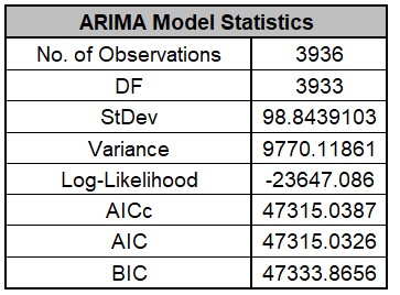
ARIMA Model Statistics and Information Criteria for Model Comparison
The ARIMA model statistics are similar to those used in Exponential Smoothing.
Log-Likelihood is related to -Ln(Sum-of-Squares Error), so is maximized. Information
Criteria AICc, AIC and BIC are calculated using -2*Log-Likelihood and incorporate a penalty
for the number of terms in the model, so smaller is better. These are used in automatic
model selection. AICc is the default Information Criterion, based on forecast error
performance with competition data.
For further details, see Information Criteria for Model
Comparison.
Open Chemical Process Concentration Series A.xlsx
(Sheet 1 tab). This is the Series A data from
Box and Jenkins, a set of 197 concentration values from a
chemical process taken at two-hour intervals. See the Run Chart,
ACF/PACF Plots, Spectral.html and Seasonal Trend
Decomposition Plots for this data.
Click SigmaXL > Time Series
Forecasting > ARIMA Forecast > Forecast. Ensure that
the entire data table is selected. If not, check Use
Entire Data Table. Click Next.
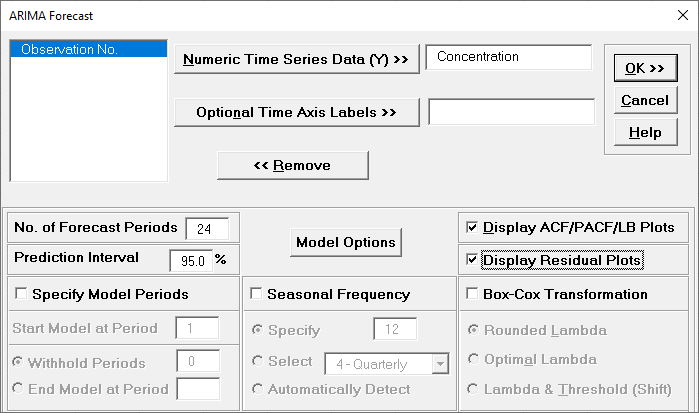
Select Concentration, click
Numeric Data
Variable (Y) >>. Check Display
ACF/PACF/LB Plots and Display Residual Plots.
Leave Specify Model Periods, Seasonal Frequency
and Box-Cox Transformation unchecked. We will
use the default No. of Forecast Periods = 24
and Prediction Interval = 95.0 %.
Optional Time Axis Labels will be displayed on the forecast
chart time axis. If used, dates for the forecast periods should
also be included, otherwise the time axis will be blank for the
forecast periods.
No. of Forecast Periods are the number of time series values
to be predicted (forecast horizon). The most accurate forecast
will be for the first predicted value (one-step-ahead).
Prediction Interval % is the confidence level for the
individual predictions. For example, a 95% prediction interval
contains a range of values which should include the actual
future value with 95% probability. The interval will get larger
the further out you predict.
Model Options opens another dialog which allows you to set
automatic options or to specify a model.
Display ACF/PACF/LB option will produce ACF
and PACF plots for the raw data as well as for the model
residuals. The LB plot is a plot of Ljung-Box test P-Values for
various lags and is used to determine if a group of
autocorrelations are significant, (i.e., the autocorrelations do
not come from a white noise series). For further details, see
Ljung-Box Test.
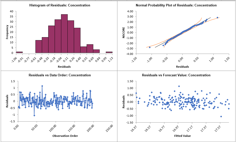
Display Residual Plots will produce a table of model residuals
and the usual model residual plots: histogram, normal probability plot, residuals
versus data order, and residuals vs forecast value. Note that if a Box-Cox
transformation is applied, the residuals are transformed so will not be equal to
forecast - actual.
Specify Model Periods are used to specify a start period, end
period or withhold sample. The withheld data is not used in model estimation, so
this is very useful for model validation and comparison. This will be used in a
later example.
Seasonal Frequency and Box-Cox Transformation
will be used in a later example.
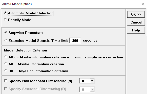
Click Model Options.
Automatic Model Selection will be used later. It is the default
selection.
Extended Model Search is described above. The Time limit may need to be increased for
seasonal models with high seasonal frequency and/or large number of observations.
Model Selection Criterion is the information criterion metric to be
used in automatic model selection. AICc is the default selection.
Specify Nonseasonal Differencing (d) = 0, 1, or 2, overrides the
automatic nonseasonal differencing. This is useful to compare models for borderline
cases that are nearly nonstationary (see Box and Jenkins).
Specify Seasonal Differencing (D) = 0 or 1, overrides the automatic
seasonal differencing. It is greyed out here because
Seasonal Frequency was unchecked in the previous dialog.
Clicking OK accepts the settings and returns you to the previous
dialog. Clicking
Cancel will cancel any changes and return you to the previous
dialog.
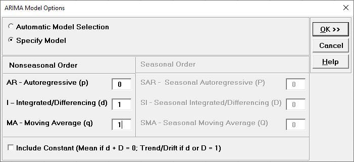
Select Specify Model.
Specify Nonseasonal Order I Integrated/Differencing
(d) = 1 and MA Moving Average (q) =
1. Leave Include Constant unchecked.
Specify Model allows you to manually specify the
Nonseasonal Order and Seasonal Order values and option
for
Include Constant (Mean if d + D = 0; Trend/Drift if d or D = 1). If d +
D = 0, then the constant term is the mean; if d or D = 1, then the constant term is a
Trend; if d + D > 1, then the constant term is quadratic or higher this is not
recommended.
Seasonal Order is greyed out because Seasonal
Frequency was unchecked in the previous dialog.
The specified ARIMA (0,1,1) is equivalent to a simple exponential smoothing model (with
slight differences due to estimation of the initial value).
Click OK to return to
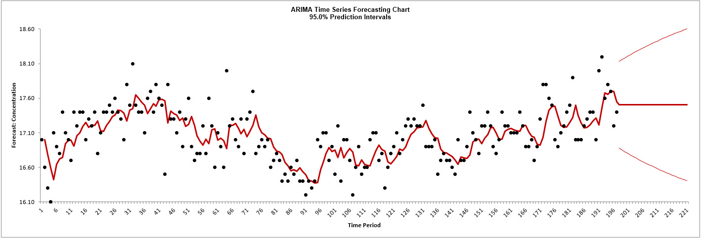
the ARIMA Forecast dialog. Click OK. The ARIMA
forecast report is given:
As expected, this is very similar to the exponential smoothing
forecast chart that was produced using the Simple
Exponential Smoothing with Additive Errors (A, N, N)
Exponentially Weighted Moving Average (EWMA) model. The
initial in-sample predicted value for ARIMA is slightly
different and starts at the second time period due to
differencing.
Scroll down to view the ARIMA Model
header:
If we had checked Specify Model Periods in the main dialog, the
start, end or withhold selection would be summarized here as
well.
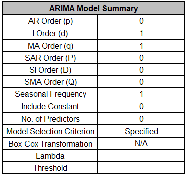
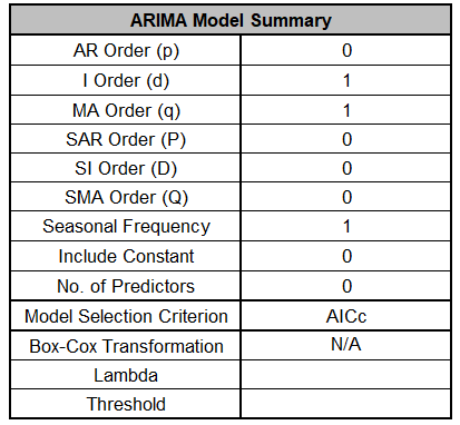
The ARIMA Model Summary is given as:
This is a summary of model information: ARIMA (0,1,1) with no
constant and no predictors. Seasonal Frequency = 1
(nonseasonal); Model Selection Criterion = Specified because
the model was user specified; and Box-Cox Transformation = N/A
because Box-Cox Transformation was unchecked.
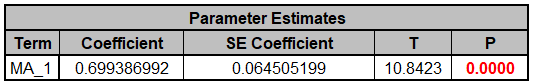
The Parameter Estimates are:
The MA_1 parameter coefficient value is approximately equal to 1 alpha = 1 - 0.2948 =
0.7052 in Exponential Smoothing
Parameter Estimates. The slight difference is due to estimation of the initial
value.
ARIMA Parameter Estimates include significance tests; P-Values < .05 are significant
and highlighted in red. This may be useful for model refinement with multiple predictors
(and will be demonstrated later). Note that for AR/MA model order selection, minimum
AICc should be used, rather than significance tests (see Kostenko, A.V. and Hyndman, R.J.).
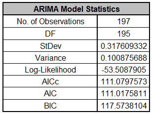
Comparing to the Exponential Smoothing Model Statistics, we see
that the StDev and Variance are approximately equal, but the
Log-Likelihood, AICc, AIC and BIC are very different. This is
due to different formulas being used in the Likelihood function.
You cannot use Information Criteria to compare ARIMA and
Exponential Smooth models to determine which model has the best
fit.
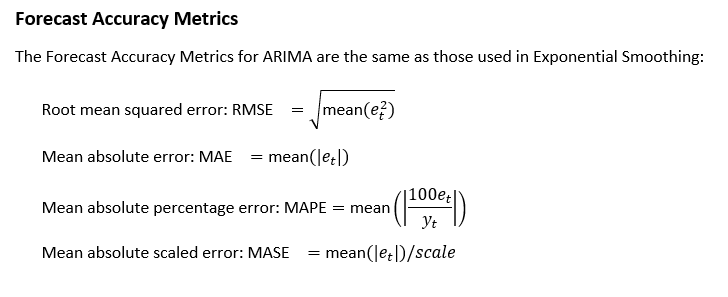
The In-Sample Forecast Accuracy metrics
are:
MASE is less than one, so it is a better forecast than would be obtained from a nave
forecast (set all forecasts to be the value of the last observation).
See Forecast Accuracy Metrics.
These are
the same forecast and prediction interval values displayed in the Forecast Chart but
provided for further analysis or charting. If Withhold Periods are specified, the
Withhold Data will be displayed as well.
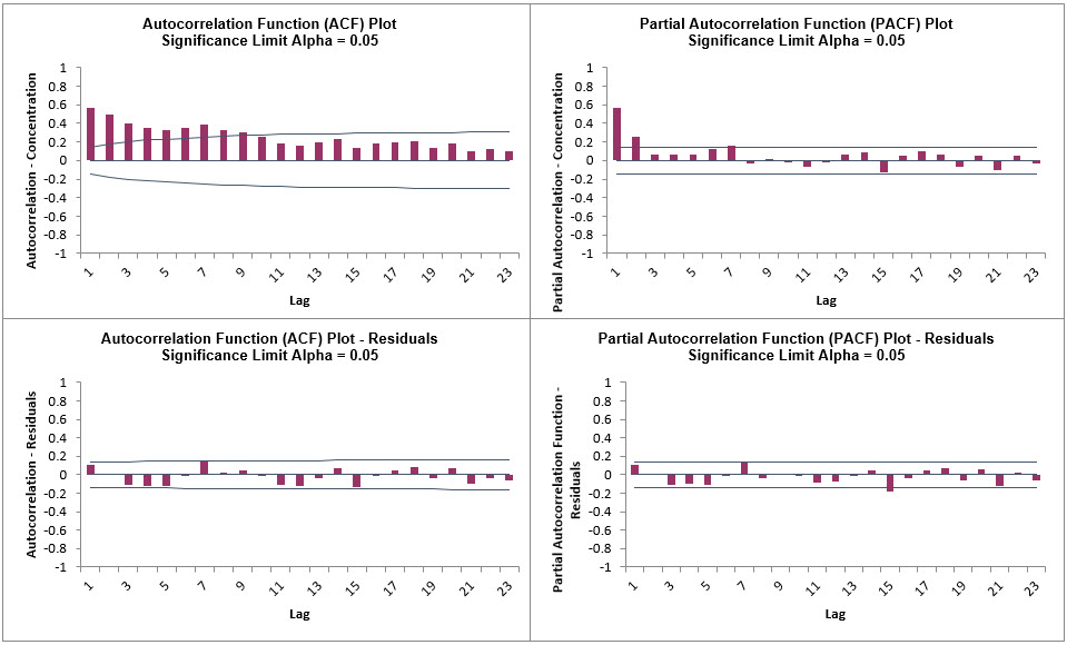
Click on the ARIMA ACF PACF
LB sheet to view the ACF/PACF/LB Plots:
These are approximately the same as what we obtained previously with Exponential Smoothing ACF/PACF/LB
Plots. We can see that all of the autocorrelation has been removed by the
exponential smoothing model (with the exception of lag 15 in the PACF), so this is a
good fit to the time series data.
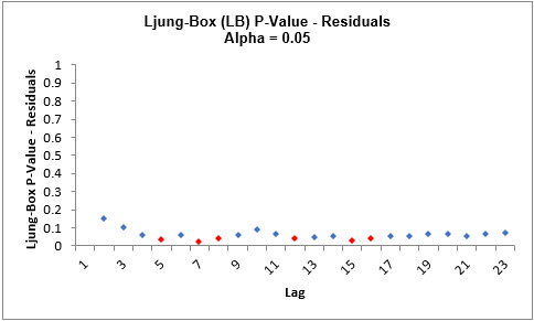
The LB plot is a plot of Ljung-Box test P-Values for various lags and is used to
determine if a group of autocorrelations are significant, (i.e., the autocorrelations do
not come from a white noise series).
For further details, see Ljung-Box Test.
The red P-Values are significant (alpha=.05) and the blue P-Values are not significant.
It is desirable that all P-Values be blue. The ACF/PACF plots indicated that almost all
of the correlation has been accounted for in the model, but the Ljung-Box plot shows
that some significant autocorrelation still remains - so the model can potentially be
improved. This does not mean that the model is a bad model, it can still be very useful
for prediction purposes, but the prediction intervals may not provide accurate
coverage.
There does appear to be fewer significant P-Values than we obtained previously with the
Exponential Smoothing LB plot,
but this may not be a practical difference, given the similarity of all the other
statistics.
Click on the ARIMA Residuals
sheet to view the Residual Plots:
The residuals are approximately normally distributed, with a
roughly straight line on the normal probability plot.
There are no obvious extreme outliers or patterns in the charts. Later, we will apply a
control chart to the residuals to formally test for significant outliers or assignable
causes.
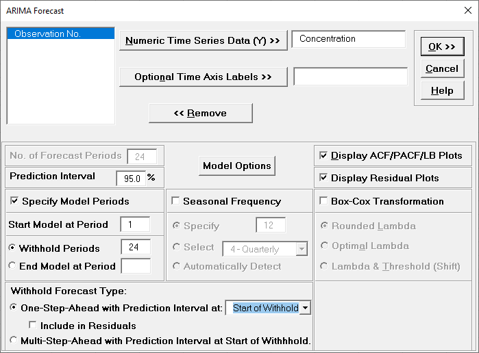
Now we will rerun ARIMA Forecast on the
Concentration data with Automatic Model Selection and Specify
Withhold Periods. Click Recall SigmaXL Dialog
menu or press F3 to Recall Last Dialog. Check
Specify Model Periods. Set Withhold
Periods = 24. We will use the default Withhold
Forecast Type: One-Step-Ahead with Prediction Interval at:
Start of Withhold.
Specify Model Periods option allows you to specify the start
and end periods used in automatic model identification and
parameter estimation. Typically, Start Model at Period is kept =
1 and Withhold Periods specifies the number of periods to be
withheld for out-of-sample testing. End Model at Period
specifies the end period, so the withhold sample size would be:
total number of observations end period.
Withhold Forecast Type: One-Step-Ahead will exclude the
withhold sample from automatic model identification and
parameter estimation, but uses the withhold data to update the
predicted one-step ahead forecast. This is useful to assess
forecast error when you only care about the short-term one-step
ahead prediction.
Withhold Forecast Type: One-Step-Ahead with Prediction
Interval at: Start of Withhold will display the prediction
interval for the duration of the withhold sample. Note that the
length of the prediction interval is determined by the number of
withhold periods, so overrides the specified No. of Forecast
Periods.
Withhold Forecast Type: One-Step-Ahead with Prediction
Interval at: End of Withhold will display the prediction
interval at the end of the withhold sample. The length of the
prediction interval is determined by the specified No. of
Forecast Periods.
Include in Residuals will treat the one-step-ahead forecast
errors as residuals (even though they were not part of the model
estimation process) and will be included in the ACF/PACF/LB
Residual Plots along with the Residuals report and graphs.
Typically, this is kept unchecked.
Withhold Forecast Type: Multi-Step-Ahead with Prediction
Interval at Start of Withhold will exclude the withhold sample
from automatic model identification and parameter estimation and
does not use the withhold data to update the predicted one-step
ahead forecast. This is useful to assess forecast error when you
are interested in a long-term forecast window (horizon). The
prediction interval will be displayed for the duration of the
withhold sample. Note that the length of the prediction interval
is determined by the number of withhold periods, so overrides
the specified No. of Forecast Periods. These forecast errors are
not included in ACF/PACF/LB Residual Plots or the Residuals
report and graphs.
Click Model Options.
Select Automatic Model Selection. We will use
the defaults: Stepwise Procedure and Model Selection Criterion:
AICc Akaike information criterion
with small sample size correction, leave Specify Nonseasonal
Differencing (d) unchecked.
Tip: When using Recall SigmaXL Dialog and if there are
no changes to the
Model Option settings, the previous settings will be used. It is not
necessary to repeat this step.
Click OK to return to
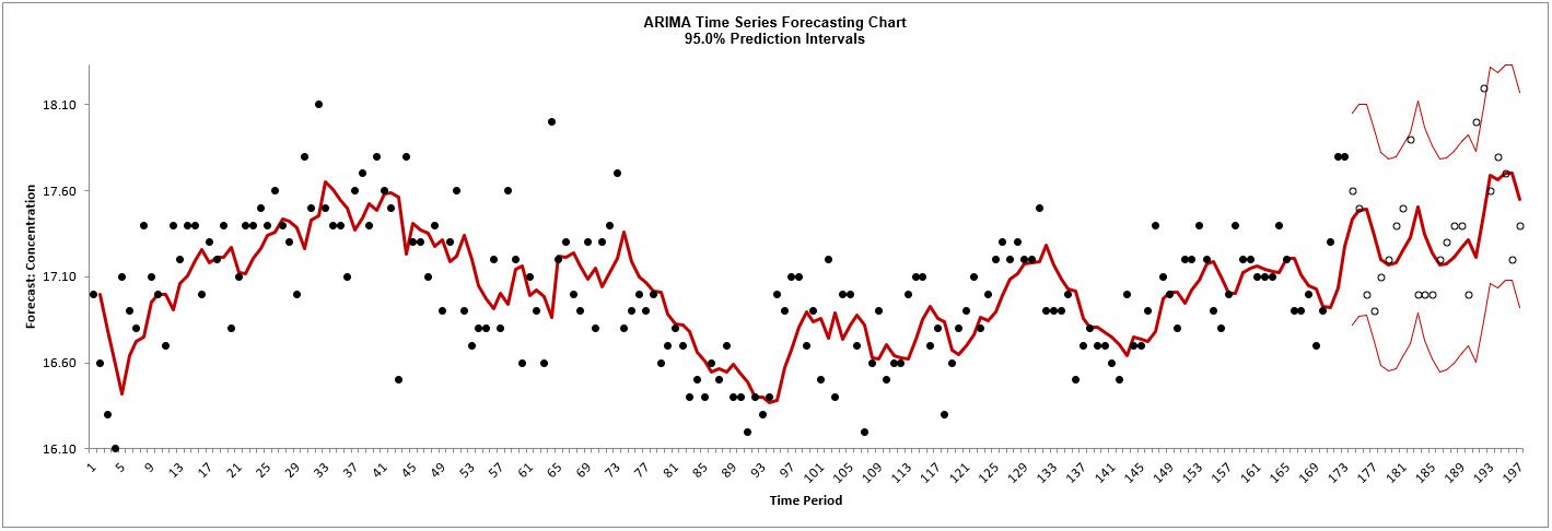
the ARIMA Forecast dialog. Click OK. The ARIMA
forecast report is given:
The blank dots are the data values in the withhold sample with a one-step-ahead forecast
and prediction intervals displayed at the start of the withhold sample.
This is very similar to the exponential smoothing forecast chart that was produced using the
Simple Exponential Smoothing with Multiplicative Errors (M, N, N) model. The initial
in-sample predicted value for ARIMA is slightly different and starts at the second time
period due to differencing.
Scroll down to view the ARIMA Model header:
The ARIMA Model Summary is given as:
The ARIMA
(0,1,1) model that we manually specified above, was also automatically selected based on
the AICc criterion.
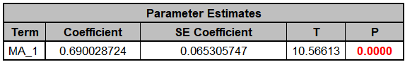
The Parameter Estimates are:
This is close to the parameter estimate obtained above (which used
all of the data).
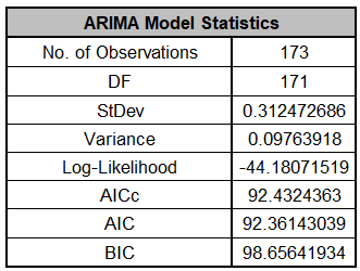
The ARIMA Model Statistics are:
These are fairly close to the model statistics obtained above
using all of the data. Here we are using only 173 of the 197 observations.
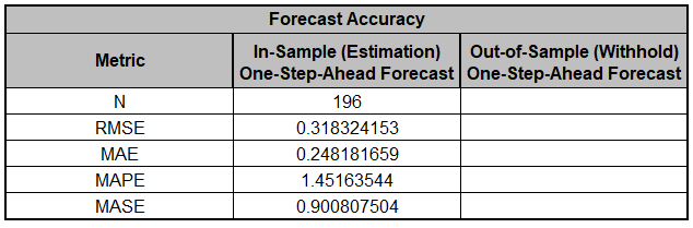
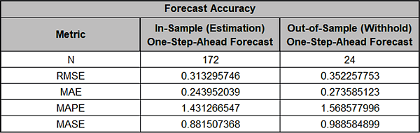
The Forecast Accuracy metrics are:
As expected, the Out-of-Sample (Withhold) One-Step-Ahead
Forecast errors are larger than the In-Sample (Estimation)
One-Step-Ahead Forecast errors.
These are very similar to the Exponential Smooth Forecast
Accuracy Metrics that were produced using the Simple Exponential
Smoothing with Multiplicative Errors (M, N, N) model. Note that
we lose one observation on the In-Sample (N=172) since we do not
have a predicted value at time period = 1 due to differencing.
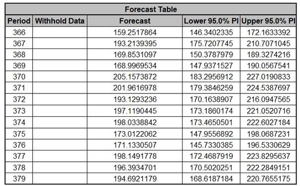
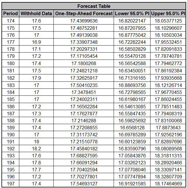
The Forecast Table is given as:
These are the same forecast and prediction interval values
displayed in the Forecast Chart, but provided for further
analysis or charting. The Withhold Data is also
displayed.
The ACF/PACF/LB Residual Plots and
Residual Plots are based on the in-sample data. The plots look
similar to the complete data above, except for the Ljung-Box
P-Values:
As was the case with exponential smoothing, the ARIMA (0,1,1) model is a better fit
to the subset than the complete data, with all P-Values being blue (> .05).
If Include in Residuals
was checked then the residuals would also include the Out-of-Sample (Withhold)
One-Step-Ahead Forecast
errors.
The above analysis can be rerun using
Withhold Forecast Type: Multi-Step-Ahead with Prediction
Interval at Start of Withhold (click Recall
SigmaXL Dialog menu or press F3 to Recall Last Dialog),
but we will not do so here. The results would be very similar to
those obtained with exponential smoothing.