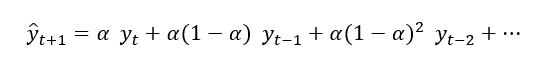
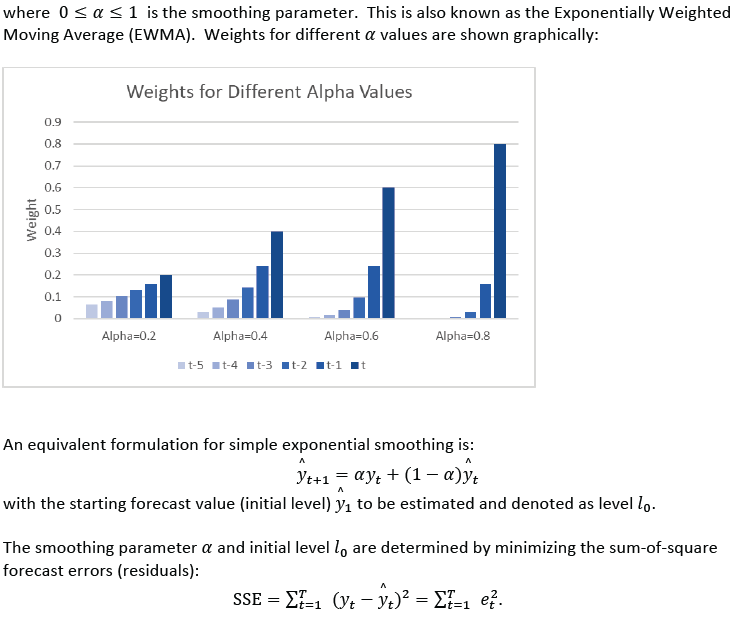
Simple Exponential Smoothing forecasts are calculated using weighted averages, where the
weights decrease exponentially as observations come from further in the past with the
smallest weights associated with the oldest observations:
Error, Trend, Seasonal (ETS) Models
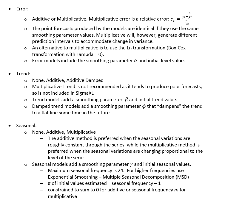
Error, Trend, Seasonal (ETS) models expand on simple exponential smoothing to accommodate
trend and seasonal components as well as additive or multiplicative errors. Simple
Exponential Smoothing is an Error Model. Error, Trend model is Holts Linear, also known as
double exponential smoothing. Error, Trend, Seasonal model is Holt-Winters, also known as
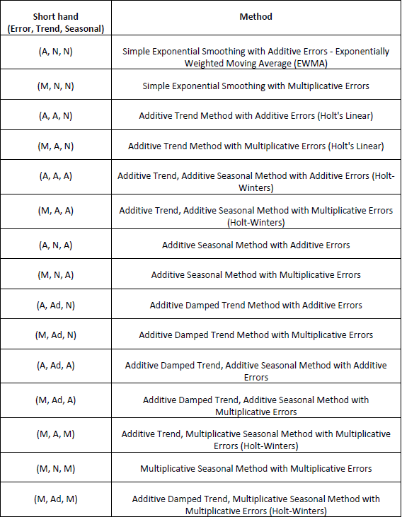
triple exponential smoothing. Rob Hyndman has developed a complete taxonomy that describes
all of the combinations of exponential smooth models in a consistent manner (see fpp2):
Exponential Smoothing Parameter Estimation, Model Statistics and Information Criteria for
Model Comparison
Model parameters are solved using nonlinear maximization of the Log-Likelihood function.
Log-Likelihood is related to -Ln(Sum-of-Squares Error). Information Criteria AICc, AIC and
BIC are calculated using -2*Log-Likelihood and incorporate a penalty for the number of terms
in the model, so smaller is better. These are used in automatic model selection. AICc is the
default Information Criterion, based on forecast error performance with competition data.
Missing Values
Exponential Smoothing handles missing values with seasonally adjusted linear interpolation.
While there is robustness against some missing values, if the number of missing values is
large then model estimation and forecast accuracy will be degraded. Upon selection of a time
series with missing values, you will see a pop-up Warning: Missing values detected.
Seasonally adjusted linear interpolation will be used.
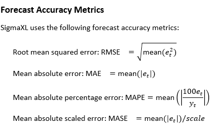
where scale is the MAE of the in-sample nave or seasonal nave forecast (set all forecasts
to be the value of the last observation/period). Note that scale for nonseasonal is
identical to MR-bar of an Individuals Moving Range chart. A scaled error is less than one if
it arises from a better forecast than the average nave/seasonal nave forecast. Conversely,
it is greater than one if the forecast is worse than the average nave forecast. MASE is
recommended over the popular MAPE, because MAPE becomes infinite if any y_t=0.
In-Sample is also referred to as the Train data. The same metrics may be applied to
Out-of-Sample (Withhold), also referred to as the Test data and may be One-Step-Ahead or
Multi-Step-Ahead. This will be demonstrated later. Out-of-Sample (Withhold) data is not used
in the model parameter estimation, so is a much better indicator of true forecast accuracy.
In-sample accuracy metrics can be biased due to overfitting. Scale is always computed using
the in-sample data.
Demo of Simple Exponential Smoothing Concentration
Open Demo of Simple Exponential Smoothing
Concentration.xlsx (Sheet 1 tab).
This is the Series A data from Box and Jenkins, a set of 197 concentration values from a
chemical process taken at two-hour intervals in Column B.
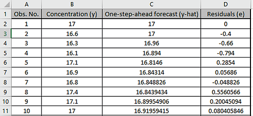
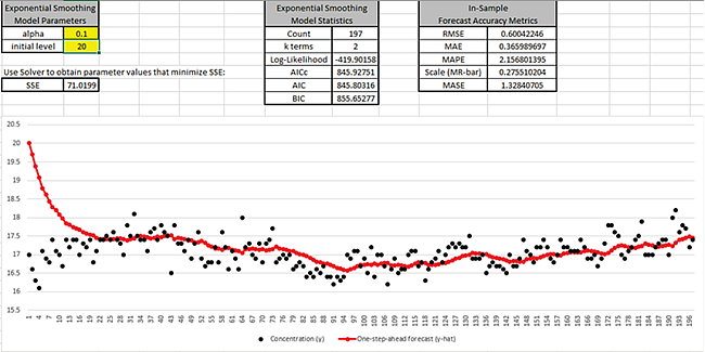
Cell G3 is the alpha smoothing parameter value, cell G4 is
the initial level. These may be manually entered or solved with Solver.
The One-step-ahead forecast is calculated as follows: C2 is the initial level value; C3
=alpha*B2+(1-alpha)*C2; C4 =alpha*B3+(1-alpha)*C3, etc.
Cell G7 is the Residuals Sum-of-Squares error and is the value to be
minimized, in order to produce the most accurate one-step-ahead forecast.
The exponential smooth model statistics are also given for later comparison to the SigmaXL
report.
The raw Concentration data are the black dots in the graph; the one-step-ahead forecast
values are the red dots.
Model Statistics and Forecast Accuracy Metrics will be discussed later.
Before we use Solver to determine the optimal alpha and initial
level values, we will manually enter some values to see how the graph changes.
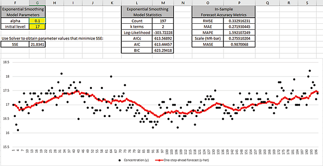
Enter alpha = 0.01 as shown:
This small value of alpha produces a smooth fit with SSE = 31.02 that is larger than what we
started with (SSE = 21.83).
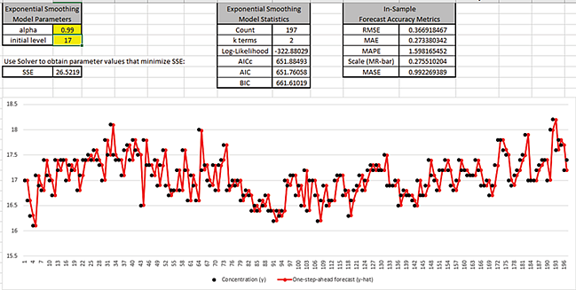
Now enter alpha = 0.99 as shown:
This large value of alpha results approximately in a nave forecast, with the one-step-ahead
forecast value equal to the previous actual. SSE = 26.52 is larger than what we started
with.
Enter alpha = 0.1 and initial level = 20 as shown:
This initial level is a poor estimate of the start value and results in SSE = 71.02. After
about 30 observations, the influence of this poor start value is negligible.
The duration for which the initial level has influence on the one-step-ahead forecast
depends on alpha, a smaller alpha would be a longer duration; a larger alpha would be a
shorter duration.
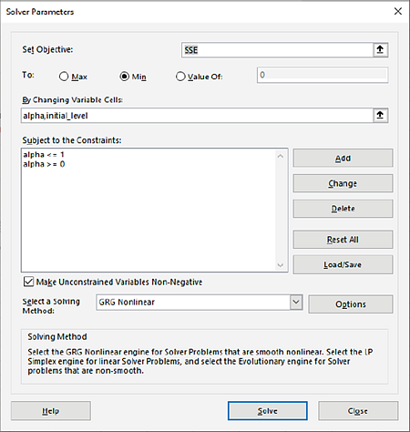
Now we will use Excels Solver to find the optimal values for alpha
and initial level. Click Data > Solver. (If the
Solver menu is not available, click
File > Options > Add-Ins. Click
Go Manage Excel Add-ins, check Solver Add-in. Click
OK. Click Data > Solver.)
The cell addresses, constraints and settings for Solver have been stored in the workbook, so
no changes are necessary. Solver will minimize cell G7 (SSE), by varying
cells G3 (alpha) and G4 (initial_level).
The solving method is GRG Nonlinear; Evolutionary could also be used but it is
slower.
Click Solve. The Solver Results dialog shows that
a solution has been found.
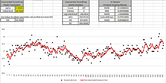
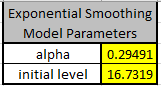
Click OK. The SSE is now 19.74; alpha value =
0.295 and initial level = 16.732.
By minimizing the residual sum-of-squares error (SSE), we have our best estimate of the
parameters to produce one-step-ahead forecast values.
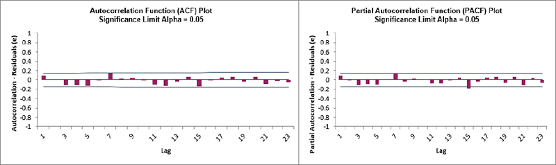
We will now produce ACF/PACF plots for the Residuals.
Select cells D1:D198 and click SigmaXL >
Time Series Forecasting > Autocorrelation (ACF/PACF)
Plots.
Click Next, Select Residuals (e), Click OK.
We can see that all of the autocorrelation has been removed by the simple exponential
smoothing model (with the exception of lag 15 in the PACF), so this is a good fit to the
time series data.
By way of comparison, these are the ACF/PACF plots for the original
Concentration data that we produced earlier.
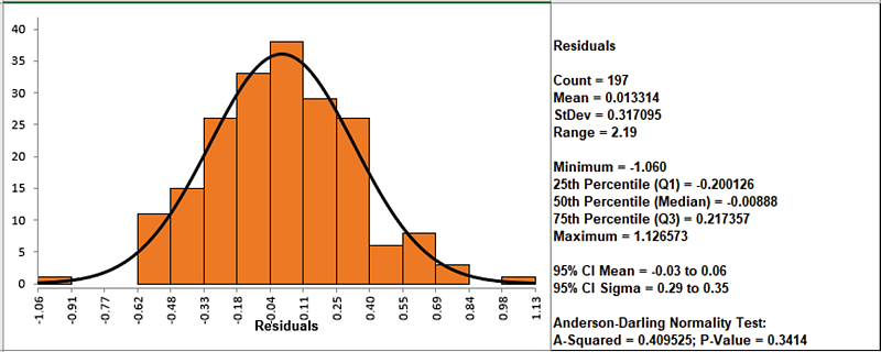
We will now have a quick look at the Residuals using a Histogram.
Select the Residuals data (D1:D198). Click SigmaXL
> Graphical Tools > Histograms and Descriptive
Statistics. Next, Select Residuals (e), Click
OK.
The residuals are normally distributed with no obvious extreme outliers.
Chemical Process Concentration - Series A
Open Chemical Process Concentration Series A.xlsx
(Sheet 1 tab). This is the Series A data from
Box and Jenkins, a set of 197 concentration values from a
chemical process taken at two-hour intervals. See the Run Chart,
ACF/PACF Plots, Spectral.html and Seasonal Trend
Decomposition Plots for this data.
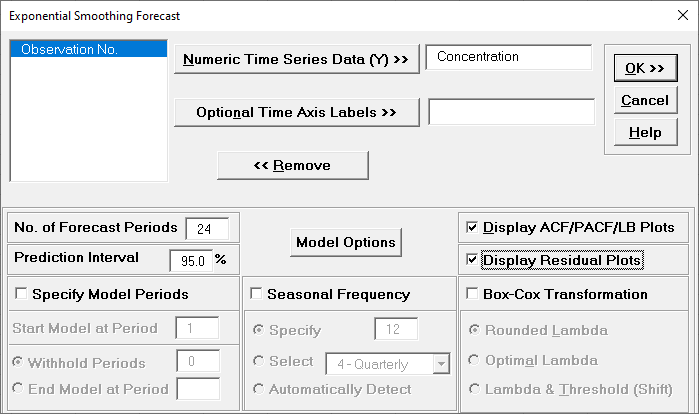
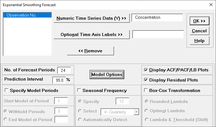
Click SigmaXL > Time Series
Forecasting > Exponential Smoothing Forecast > Forecast. Ensure that
the entire data table is selected. If not, check Use
Entire Data Table. Click Next.
Select Concentration, click
Numeric Data
Variable (Y) >>. Check Display
ACF/PACF/LB Plots and Display Residual Plots.
Leave Specify Model Periods, Seasonal Frequency
and Box-Cox Transformation unchecked. We will
use the default No. of Forecast Periods = 24
and Prediction Interval = 95.0 %.
Optional Time Axis Labels will be displayed on the forecast
chart time axis. If used, dates for the forecast periods should
also be included, otherwise the time axis will be blank for the
forecast periods.
No. of Forecast Periods are the number of time series values
to be predicted (forecast horizon). The most accurate forecast
will be for the first predicted value (one-step-ahead).
Prediction Interval % is the confidence level for the
individual predictions. For example, a 95% prediction interval
contains a range of values which should include the actual
future value with 95% probability. The interval will get larger
the further out you predict.
Model Options opens another dialog which allows you to set automatic
options or to specify a model.
Display ACF/PACF/LB option will produce ACF
and PACF plots for the raw data as well as for the model
residuals. The LB plot is a plot of Ljung-Box test P-Values for
various lags and is used to determine if a group of
autocorrelations are significant, (i.e., the autocorrelations do
not come from a white noise series).
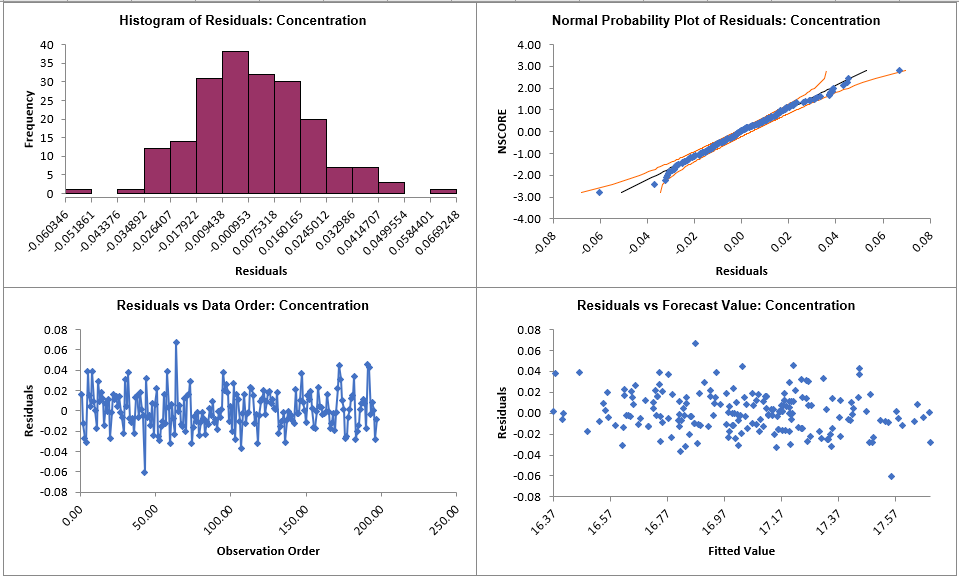
Display Residual Plots will produce a table of model residuals and the
usual model residual plots: histogram, normal probability plot, residuals versus data order,
and residuals vs forecast value. Note that if a Box-Cox transformation is applied, the
residuals are transformed so will not be equal to forecast - actual.
Specify Model Periods are used to specify a start period, end period or
withhold sample. The withheld data is not used in model estimation, so this is very useful
for model validation and comparison. This will be used in a later example.
Seasonal Frequency and Box-Cox Transformation will be
used in a later example.
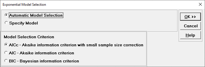
Click Model Options.
Automatic Model Selection will be used later. It is the default
selection.
Model Selection Criterion is the information criterion metric to be used
in automatic model selection. AICc is the default selection.
Clicking OK accepts the settings and returns you to the previous dialog.
Clicking
Cancel will cancel any changes and return you to the previous dialog.
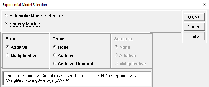
Select Specify Model.
Specify Model allows you to manually specify
the Error-Trend-Seasonal model. Seasonal options are greyed out
because the Seasonal Frequency option in the
main dialog is unchecked. A summary description of the model is
also given. This will be included in the forecast report.
We will use the default Error:
Additive and Trend: None, which is a
simple exponential smoothing model, the same as was demonstrated
previously. Click OK to return to the
Exponential Smoothing Forecast dialog. Click OK.
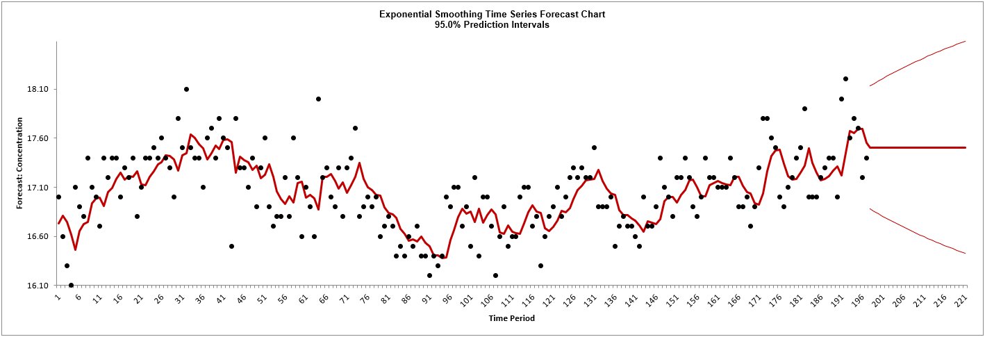
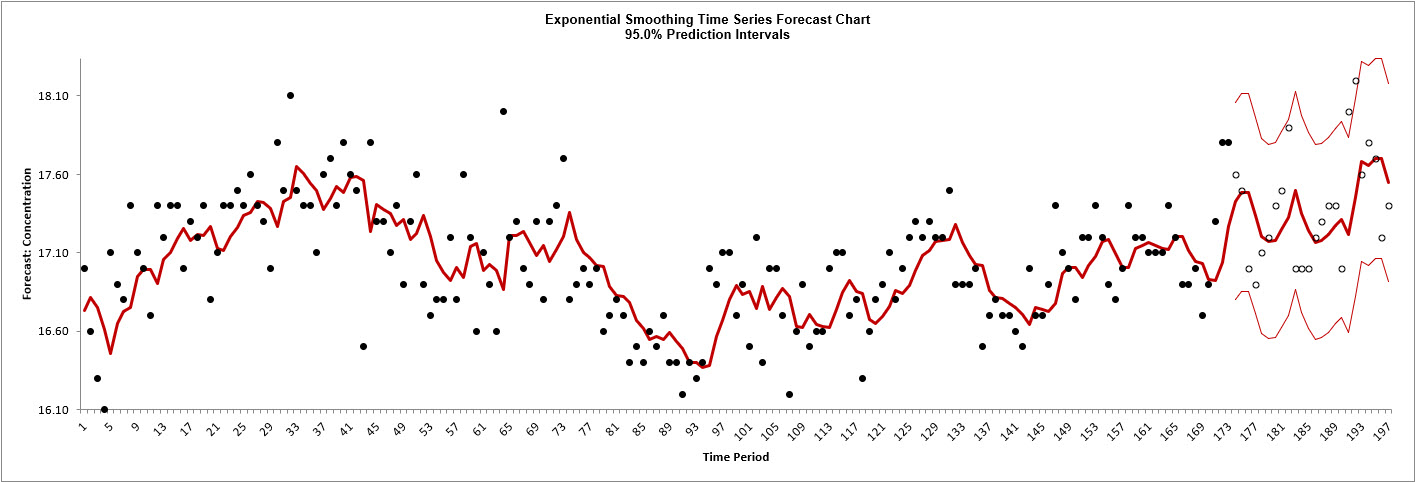
The exponential smoothing forecast chart is given:
This is very similar to the exponential smooth plot demonstrated
above, showing the raw Concentration data (black) and
one-step-ahead forecast values (red), but with the addition of a
24-period forecast and the 95% prediction interval.
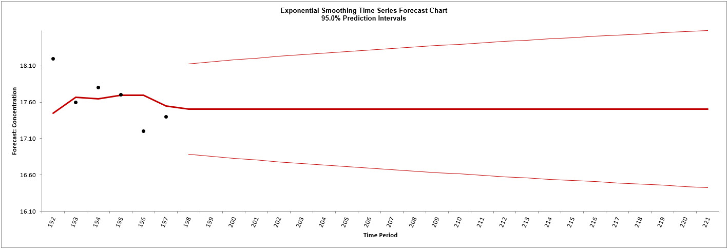
You can zoom in to view the last 30
points on the Forecast Chart. Click SigmaXL Chart Tools
> Show Last 30 Data Points.
To restore the chart, click
SigmaXL Chart Tools > Show All Data Points.
You can also scroll through the data.
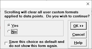
Click SigmaXL Chart Tools > Enable Scrolling
You are prompted with a warning message that custom formatting
on the chart will be cleared:
You can avoid seeing this warning by checking Save this
choice as default and do not show this form again.
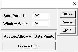
Click OK. The scroll
dialog appears allowing you to specify the Start Period
and Window Width:
At any point, you can click Restore/Show All Data Points
or Freeze Chart. Freezing the chart will remove
the scroll and unload the dialog. The scroll dialog will also
unload if you change worksheets. To restore the dialog, click
SigmaXL Chart Tools > Enable Scrolling.
Click OK. A scroll bar
appears beneath the forecast chart. You can also change the
Start Subgroup and Window Width
and Update.
You can scroll through by clicking to the right or left, with
the specified window width of 20. Click left once to view the
chart as shown.
Click Cancel to exit
the scroll dialog.
Scroll down to view the Exponential
Smoothing Model header:
The model Simple Exponential Smoothing with Additive Errors (A,
N, N) Exponentially Weighted Moving Average (EWMA) is the user
specified model. This is the same model information that was
displayed in the Model Selection dialog.
If we had checked Specify Model Periods in the main dialog, the
start, end or withhold selection would be summarized here as
well.
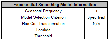
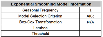
The Exponential Smoothing Model
Information is given as:
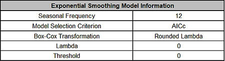
This is a summary of model information with Seasonal Frequency =
1 (nonseasonal); Model Selection Criterion = Specified because
the model was user specified; and Box-Cox Transformation = N/A
because Box-Cox Transformation was unchecked.
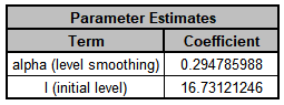
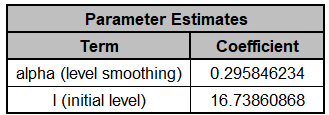
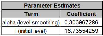
The Parameter Estimates are:
The parameter estimates closely match the values obtained
earlier in the demonstration using Solver:
The slight differences in parameter results are due to
differences in optimization method.
The results match those given in the demonstration using Solver:
The equations may be viewed by clicking on the Demo
cells
M5, M6, M7 or M8.
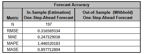
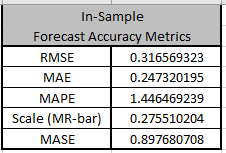
The In-Sample Forecast Accuracy metrics
are:
MASE is less than one, so it is a better forecast than would be
obtained from a nave forecast (set all forecasts to be the
value of the last observation). See Forecast Accuracy Metrics.
The results closely match those given in the demonstration using
Solver:
The equations may be viewed by clicking on the Demo
cells
P3 to P7.
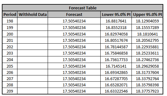
The Forecast Table is given as:
These are the same forecast and prediction interval
values displayed in the Forecast Chart but provided for further analysis or charting. If
Withhold Periods are specified, the Withhold Data will be displayed as well.
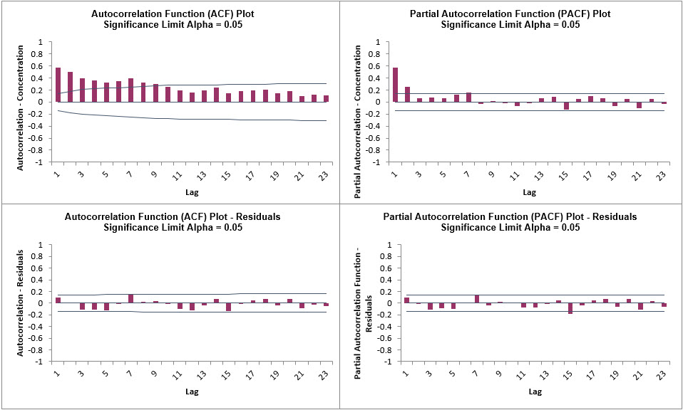
Click on the Exp. Smooth. ACF
PACF LB sheet to view the ACF/PACF/LB Plots:
These match the plots that we obtained previously in the Demo.
We can see that all of the autocorrelation has been removed by
the exponential smoothing model (with the exception of lag 15 in
the PACF), so this is a good fit to the time series data.
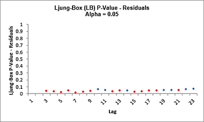
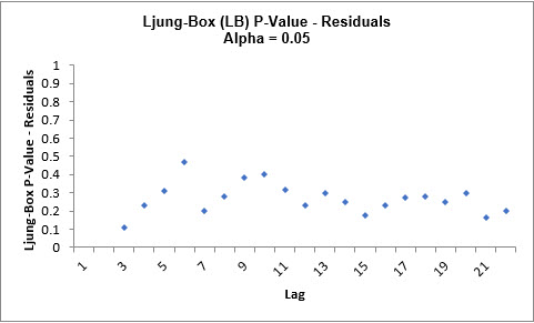
The LB plot is a plot of Ljung-Box test P-Values for various lags and is used to
determine if a group of autocorrelations are significant, (i.e., the autocorrelations do
not come from a white noise series).
For further details, see Ljung-Box Test.
The red P-Values are significant (alpha=.05) and the blue P-Values are not significant.
It is desirable that all P-Values be blue. The ACF/PACF plots indicated that almost all
of the correlation has been accounted for in the model, but the Ljung-Box plot shows
that some significant autocorrelation still remains - so the model can potentially be
improved. This does not mean that the model is a bad model, it can still be very useful
for prediction purposes, but the prediction intervals may not provide accurate
coverage.
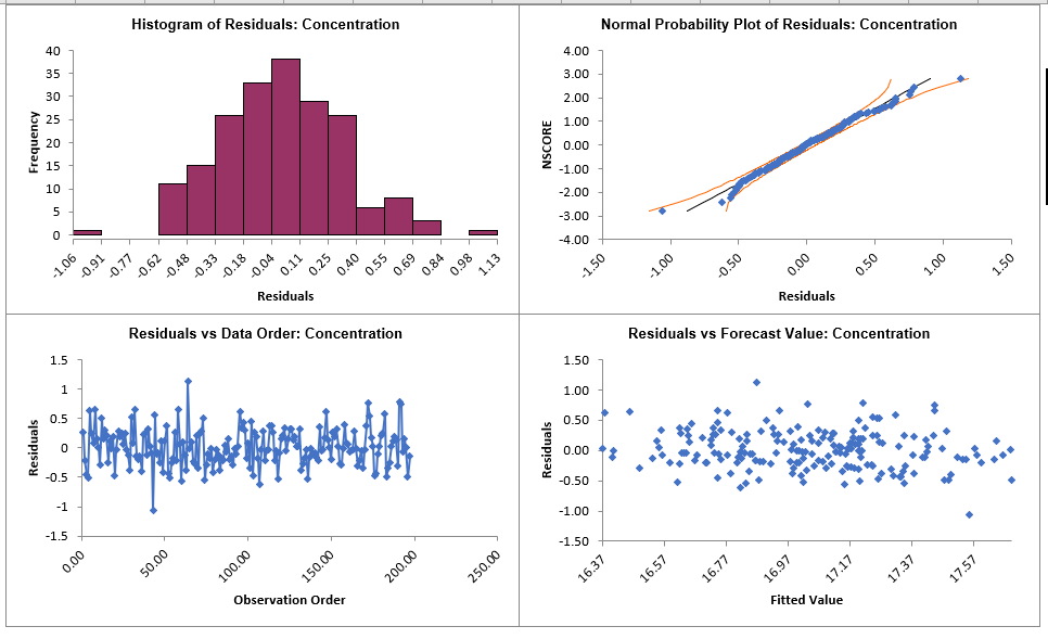
Click on the Exp. Smoothing Residuals
sheet to view the Residual Plots:
These residual plots are the same as used in SigmaXLs Multiple
Regression. The histogram matches what we obtained in the Demo
(the normal curve is not applied here). The residuals are
approximately normally distributed, with a roughly straight line
on the normal probability plot. There are no obvious extreme
outliers or patterns in the charts. Later, we will apply a
control chart to the residuals to formally test for significant
outliers or assignable causes.
Now we will rerun Exponential Smoothing
on the Concentration data but use Automatic Model Selection.
Click Recall SigmaXL Dialog menu or press
F3 to
Recall Last Dialog.
Click Model Options.
Select Automatic Model Selection. We will use
the default Model Selection Criterion: AICc Akaike
information criterion with small sample size correction.
Click OK to return to
the Exponential Smoothing Forecast dialog. Click OK. The
exponential smoothing forecast report is given.
Scroll down to view the Exponential
Smoothing Model header:
The model Simple Exponential Smoothing with
Multiplicative Errors (M, N, N) was selected as the
best fit for the Concentration data based on the AICc criterion.
The point forecasts produced by the Multiplicative and Additive
models are identical if they use the same smoothing parameter
values. Multiplicative will, however, generate different
prediction intervals to accommodate change in variance.
The Exponential Smoothing Model
Information is given as:
This is a summary of model information with Seasonal
Frequency = 1 (nonseasonal); Model Selection Criterion = AICc and Box-Cox
Transformation = N/A because Box-Cox Transformation was unchecked.
The Parameter Estimates are:
These are fairly close to the parameter estimates
obtained above using the additive model.
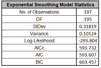
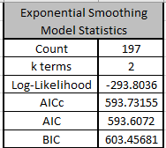
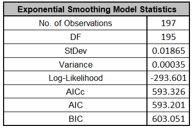
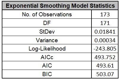
The Exponential Smoothing Model Statistics are:
The Log-Likelihood, AICc, AIC and BIC are close to the
values obtained above
using the additive model, but the Log-Likelihood is slightly
higher giving a lower AICc, so multiplicative was selected as
the best model. Note however that the StDev and Variance are
very different. This difference is due to the multiplicative
residuals being relative errors:
The In-Sample Forecast Accuracy metrics, Forecast Table and
ACF/PACF/LB Plots for multiplicative are very close to the
additive model. The multiplicative residual plots look the same,
but note the different scale due to the relative errors.
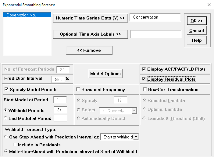
Now we will rerun Exponential Smoothing on the Concentration
data with Automatic Model Selection, but will use Specify
Withhold Periods. Click Recall SigmaXL Dialog menu or press F3
to Recall Last Dialog. Check Specify Model Periods. Set Withhold
Periods = 24 (i.e., we will forecast 24 periods and compare
against the withheld actual). We will use the default Withhold
Forecast Type: One-Step-Ahead with Prediction Interval at:Start
of Withhold.
Specify Model Periods option allows you to specify the start and end
periods used in automatic model identification and parameter estimation. Typically,
Start Model at Period is kept = 1 and Withhold Periods specifies the
number of periods to be withheld for out-of-sample testing.
End Model at Period specifies the end period, so the withhold sample
size would be: total number of observations end period.
Withhold Forecast Type: One-Step-Ahead will exclude the withhold
sample from automatic model identification and parameter estimation, but uses the
withhold data to update the predicted one-step ahead forecast. This is useful to assess
forecast error when you only care about the short-term one-step ahead
prediction.
Withhold Forecast Type: One-Step-Ahead with Prediction Interval at:
Start of Withhold will display the prediction interval for the duration of the
withhold sample. Note that the length of the prediction interval is determined by the
number of withhold periods, so overrides the specified
No. of Forecast Periods.
Withhold Forecast Type: One-Step-Ahead with Prediction Interval at:
End of Withhold will display the prediction interval at the end of the withhold
sample. The length of the prediction interval is determined by the specified
No. of Forecast Periods.
Include in Residuals will treat the one-step-ahead forecast errors as
residuals (even though they were not part of the model estimation process) and will be
included in the ACF/PACF/LB Residual Plots along with the Residuals report and graphs.
Typically, this is kept unchecked.
Withhold Forecast Type: Multi-Step-Ahead with Prediction Interval at Start of
Withhold will exclude the withhold sample from automatic model
identification and parameter estimation and does not use the withhold data to update the
predicted one-step ahead forecast. This is useful to assess forecast error when you are
interested in a long-term forecast window (horizon). The prediction interval will be
displayed for the duration of the withhold sample. Note that the length of the
prediction interval is determined by the number of withhold periods, so overrides the
specified
No. of Forecast Periods. These forecast errors are not included in
ACF/PACF/LB Residual Plots or the Residuals report and graphs.
Click Model Options. Select Automatic Model Selection.
We will
use the default Model Selection Criterion: AICc Akaike
information criterion with small sample size correction.
Tip: When using Recall SigmaXL Dialog, and if there
are no changes to the
Model Option settings, the previous settings will be used. It is not
necessary to repeat this step.
Click OK to return to the Exponential Smoothing
Forecast dialog. Click OK. The exponential
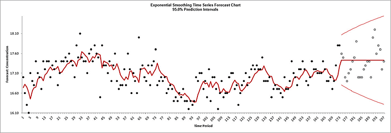
smoothing forecast report is given:
The blank dots are the data values in the withhold
sample with a one-step-ahead forecast and prediction intervals displayed at the start of
the withhold sample.
Scroll down to view the Exponential Smoothing Model header:
As with the complete data, the model
Simple Exponential Smoothing with Multiplicative Errors (M, N, N) was
selected as the best fit for the Concentration data based on the AICc criterion. The
header also includes the number of specified withhold periods.
The Parameter Estimates are:
These are close to the parameter estimates obtained above (which
used all of the data with the multiplicative model).
The Exponential Smoothing Model Statistics are:
These are fairly close to the model statistics obtained above (which
used all of the data with the multiplicative model). Here we are using only 173 of the
197 observations.
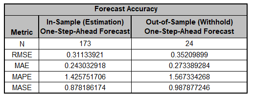
The Forecast Accuracy metrics are:
As expected, the
Out-of-Sample (Withhold) One-Step-Ahead Forecast errors are larger than
the
In-Sample (Estimation) One-Step-Ahead Forecast errors.
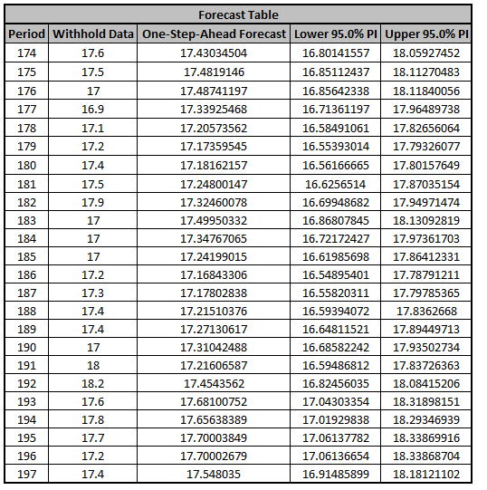
The Forecast Table is given as:
These are the same forecast and prediction interval
values displayed in the Forecast Chart, but provided for further analysis or charting.
The
Withhold Data is also displayed.
The ACF/PACF/LB Residual Plots and Residual Plots are based on
the in-sample data. The plots look similar to the complete data
above, except for the Ljung-Box P-Values:
The
Simple Exponential Smoothing with Multiplicative Errors (M, N, N) model
is a better fit to the subset than the complete data, with all P-Values being blue (>
.05).The
Simple Exponential Smoothing with Multiplicative Errors (M, N,
N) model is a better fit to the subset than the complete data,
with all P-Values being blue (> .05).
If Include in Residuals was checked then the
residuals would also include the Out-of-Sample
(Withhold) One-Step-Ahead Forecast errors.
Now we will rerun Exponential Smoothing on the Concentration
data, but use Multi-Step-Ahead for the Withhold Forecast. Click
Recall SigmaXL Dialog menu or press F3 to recall last
dialog.
Select Withhold Forecast Type: Multi-Step-Ahead with Prediction
Interval at Start of Withhold.
Click OK. The exponential smoothing forecast
report is given:
The blank dots are the data values in the withhold sample with a multi-step forecast
and prediction intervals displayed at the start of the withhold sample.
The Forecast Accuracy metrics are:
As expected, the
Out-of-Sample (Withhold) Multi-Step-Ahead Forecast errors are larger
than the
In-Sample (Estimation) One-Step-Ahead Forecast errors and the
Out-of-Sample (Withhold) One-Step-Ahead Forecast errors above.
Monthly Airline Passengers - Series G
Open Monthly Airline Passengers - Series G.xlsx (Sheet 1 tab). This is the Series G data from Box and Jenkins, monthly total international airline passengers for January 1949 to December 1960.
See the Run Chart, ACF/PACF Plots, Spectral.html and Seasonal Trend Decomposition Plots for this data.
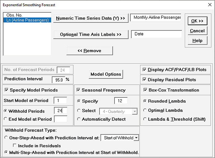
Click SigmaXL > Time Series Forecasting > Exponential Smoothing Forecast > Forecast. Ensure that the entire data table is selected. If not, check Use Entire Data Table. Click Next.
Select Monthly Airline Passengers, click Numeric Time Series Data (Y) >>.
Select Date, click Optional Time Axis Labels >>.
Check Display ACF/PACF/LB Plots and Display Residual Plots. Check Specify Model Periods.
Set Withhold Periods = 24 (i.e., we will forecast 24 months and compare to withheld actual).
Select Withhold Forecast Type: Multi-Step-Ahead with Prediction Interval at Start of Withhold.
Check Seasonal Frequency with Specify = 12.
Check Box-Cox Transformation and select Rounded Lambda (selected because the Run Chart showed an increase in the seasonal variance over time).
We will use the default Prediction Interval = 95.0%.
Withhold Forecast Type: Multi-Step-Ahead with Prediction Interval at Start of Withhold will exclude the withhold sample from automatic model identification and parameter estimation and does not use the withhold data to update the predicted one-step ahead forecast.
This is useful to assess forecast error when you are interested in a long-term forecast window (horizon).
The prediction interval will be displayed for the duration of the withhold sample.
Note that the length of the prediction interval is determined by the number of withhold periods, so overrides the specified
No. of Forecast Periods.
Seasonal Frequency Specify is used to specify the seasonal frequency.
Note that Exponential Smoothing is limited to a maximum seasonal frequency of 24. For higher frequencies use Exponential Smoothing Multiple Seasonal Decomposition (MSD)
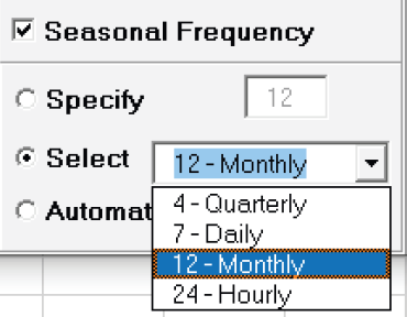
Seasonal Frequency Select gives a drop-down list of commonly used seasonal frequencies:
Seasonal Frequency Automatically Detect should be used if uncertain what the seasonal frequency value is (or do a Spectral.html prior to the Seasonal Trend Decomposition Plots). If detected frequency is > 24, 1 is returned.
If that occurs, please use Exponential Smoothing Multiple Seasonal Decomposition (MSD).
Box-Cox Transformation with Rounded Lambda will select Lambda = 0 (Ln), 0.5 (SQRT) or 1 (Untransformed).
Threshold (Shift) is computed automatically if the time series data includes 0 or negative values, otherwise it is 0.
Box-Cox Transformation with Optimal Lambda uses the range of 0 to 1 for Lambda.
Threshold is computed automatically if the time series data includes 0 or negative values.
Box-Cox Transformation with Lambda & Threshold (Shift) if left blank, will compute optimal lambda and threshold.
The user may also specify Lambda and Threshold.
Lambda may be specified outside of the 0 to 1 range, but practically for time series analysis, should be limited to -1 to 2.
Threshold is typically 0, but if the time series data includes 0 or negative values, a negative threshold value should be entered that is smaller than the minimum data value.
This value will be subtracted from the data resulting in positive time series values.
Click Model Options.
We will use the default Automatic Model Selection with AICc as the Model Selection Criterion.
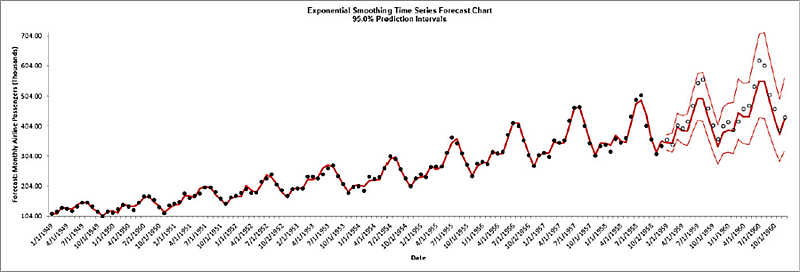
Click OK to return to the Exponential Smoothing Forecast dialog. Click OK. The exponential smoothing forecast report is given:
The blank dots are the data values in the withhold sample with a multi-step forecast and prediction intervals displayed at the start of the withhold sample.
Note that the data has been transformed using Box-Cox, but the inverse transformation is applied to produce this chart with the original units.
Scroll down to view the Exponential Smoothing Model header:
The model Additive Trend,
Additive Seasonal Method with Additive Errors (Holt-Winters) (A, A, A) was automatically selected as the best fit for the Box-Cox transformed Airline Passenger data based on the AICc criterion. Note that multiplicative models are not considered when
Box-Cox Transformation is checked. If a multiplicative model was desired, then one could manually transform the data and model Ln(Airline Passengers) with
Box-Cox Transformation unchecked.
The header also includes the number of specified withhold periods.
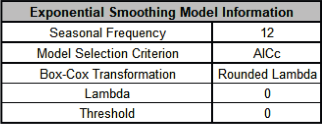
The Exponential Smoothing Model Information is given as:
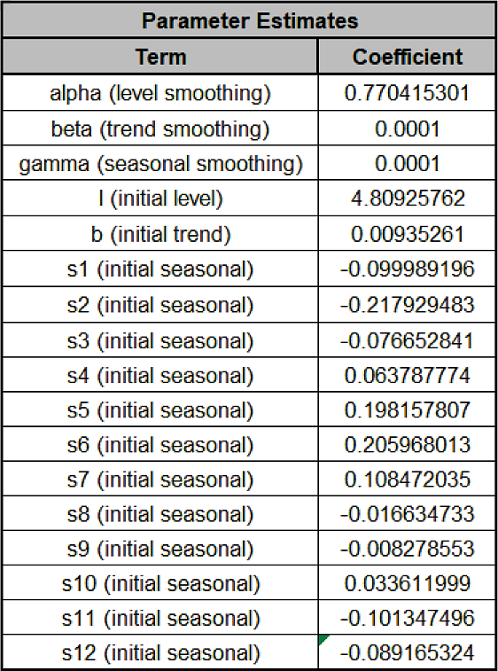
The Parameter Estimates are:
Error includes the smoothing parameter alpha and initial level value (l). The error is additive, but on the Ln transformed data.
Trend adds a smoothing parameter (beta) and initial trend value (b).
Seasonal adds a smoothing parameter (gamma) and initial seasonal values (s1 to s12), constrained to sum to zero for additive.
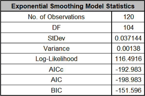
The Exponential Smoothing Model Statistics are:
The number of observations, n = 144 24 (withhold) = 120
Degrees of freedom (DF) = 120 (n) 16 (terms in the model, excluding s12) = 104
Note that the model statistics are based on the Ln transformed data, not the original data.
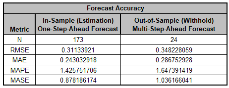
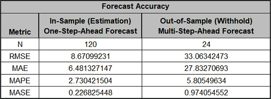
The Forecast Accuracy metrics are:
As expected, the Out-of-Sample (Withhold) Multi-Step-Ahead Forecast errors are larger than the In-Sample (Estimation) One-Step-Ahead Forecast errors.
Note, if we were primarily interested in a short term one-step ahead forecast, then we would have selected Withhold Forecast Type: One-Step-Ahead and this table would show Out-of-Sample (Withhold) One-Step-Ahead Forecast errors.
Forecast Accuracy metrics are calculated using the actual raw data versus inverse transformed forecast as displayed in the Forecast Chart and Table, so allows comparison across all model types and transformations.
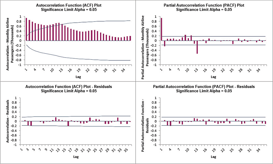
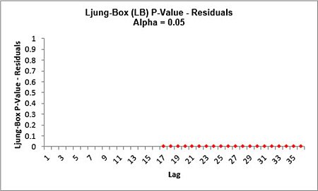
Click on the Exp. Smooth. ACF PACF LB sheet to view the ACF/PACF/LB Plots:
The ACF/PACF Residuals Plots indicate that almost all of the autocorrelation has been accounted for in the model, but the Ljung-Box plot shows that significant autocorrelation still remains (the red P-Values are significant at alpha=.05) - so the model can potentially be improved.
This does not mean that the model is a bad model, it can still be very useful for prediction purposes, but the prediction intervals may not provide accurate coverage.
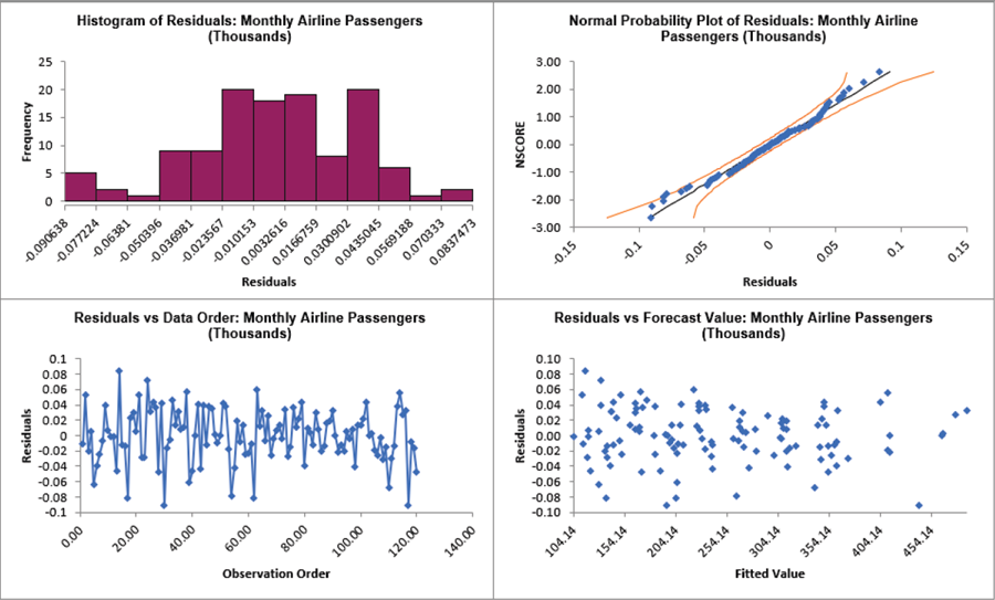
Click on the Exp. Smoothing Residuals sheet to view the Residual Plots:
The residuals are approximately normally distributed, with a roughly straight line on the normal probability plot.
There are no obvious extreme outliers or patterns in the charts.
Note that the residuals are based on the Ln transformed data, not the original data.
The Exponential Smoothing Model Information to the right of the plots shows the Box-Cox Transformation information.