Chemical Process Concentration - Series A

1. Open Chemical Process Concentration Series A.xlsx (Sheet 1 tab). This is the Series A data from Box and Jenkins, a set of 197 concentration values from a chemical process taken at two-hour intervals.
2. Click SigmaXL > Time Series Forecasting > Spectral.html. Ensure that the entire data table is selected. If not, Use Entire Data Table. Click Next.
3. Click Concentration, click Numeric Time Series Data (Y) >>.

   
   

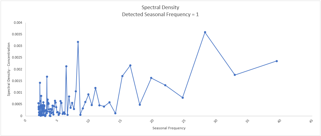
4. Click OK. A Spectral.html for Concentration is produced. The detected seasonal frequency is 1, which means that it is a nonseasonal process. The peak at 28 does not have enough seasonal strength to be considered for use as seasonal frequency in a time series model.



Monthly Airline Passengers - Series G

5. Open Monthly Airline Passengers - Series G.xlsx (Sheet 1 tab). This is the Series G data from Box and Jenkins, monthly total international airline passengers for January 1949 to December 1960.
6. Click SigmaXL > Time Series Forecasting > Spectral.html. Ensure that the entire data table is selected. If not, check Use Entire Data Table. Click Next.
7. Select Ln(Airline Passengers), click Numeric Time Series Data (Y) >>.
   
8. Click OK. A Spectral.html for Ln(Airline Passengers) is produced.
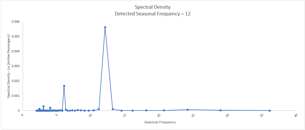
   As expected, the detected seasonal frequency for the monthly data is 12. The peak at 6 does not have enough seasonal strength to be considered as a second seasonal frequency.
   
   

   Daily Electricity Demand with Predictors ElecDaily

9. Open Daily Electricity Demand with Predictors ElecDaily.xlsx (Sheet 1 tab). This is daily electricity demand (GW) for the state of Victoria, Australia, every day during 2014 (Hyndman, fpp2). This data has a seasonal frequency = 7 (observations per week).
10. Click SigmaXL > Time Series Forecasting > Spectral.html. Ensure that the entire data table is selected. If not, check Use Entire Data Table. Click Next.
11. Select Demand, click Numeric Time Series Data (Y) >>.
    
12. Click OK. A Spectral.html for Demand is produced.
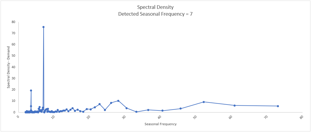
    As expected, the detected seasonal frequency for the daily data is 7.
    
    

    Sales with Indicator - Modified Series M

13. Open Sales with Indicator - Modified Series M.xlsx. (Sheet 1 tab). This is modified Series M data from Box and Jenkins, with 50 quarters of corporate sales values along with a leading indicator. The data is treated as nonseasonal, as done in Box and Jenkins.
14. Click SigmaXL > Time Series Forecasting > Spectral.html. Ensure that the entire data table is selected. If not, check Use Entire Data Table. Click Next.
15. Select Sales, click Numeric Time Series Data (Y) >>.
    
16. Click OK. A Spectral.html for Sales is produced.
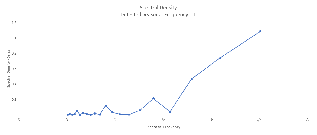
    The detected seasonal frequency is 1, which means that it is confirmed to be a nonseasonal process. The peak at 10 does not have enough seasonal strength to be considered for use as seasonal frequency in a time series model.
    
    

    Half-Hourly Multiple Seasonal Electricity Demand Taylor

17. Open Half-Hourly Multiple Seasonal Electricity Demand - Taylor.xlsx (Sheet 1 tab). This is halfhourly electricity demand (MW) in England and Wales from Monday, June 5, 2000 to Sunday, August 27, 2000 (taylor, R forecast). This data has multiple seasonality with frequency = 48 (observations per day) and 336 (observations per week), with a total of 4032 observations.
18. Click SigmaXL > Time Series Forecasting > Spectral Density Plot. Ensure that the entire data table is selected. If not, check Use Entire Data Table. Click Next.
19. Select Demand, click Numeric Time Series Data (Y) >>.
    
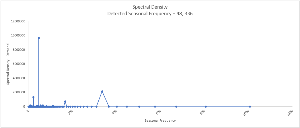
20. Click OK. A Spectral.html for Demand is produced. The detected multiple seasonal frequency is confirmed as 48, 336.
    
    
    
    The Spectral.html is used to identify the dominant integer seasonal frequency in time series data using spectral analysis with fast Fourier transforms. The algorithm used here is the same as used in the forecast model option to automatically detect seasonal frequency. If there is multiple seasonality, up to three integer frequencies will be identified. If the peak frequency is not an integer, it is rounded.
    
    The Y axis is Spectral Density, the X axis is Seasonal Frequency. The Spectral.html is also known as a Periodogram. Note that SigmaXLs use of the term seasonal frequency is the inverse of what is typically used in Fourier transforms seasonal period, as discussed in the Introduction.