Seasonal Trend Decomposition Plots

Chemical Process Concentration - Series A

1. Open Chemical Process Concentration Series A.xlsx (Sheet 1 tab). This is the Series A data from Box and Jenkins, a set of 197 concentration values from a chemical process taken at two-hour intervals.


2. Click SigmaXL > Time Series Forecasting > Seasonal Trend Decomposition Plots. Ensure that the entire data table is selected. If not, Use Entire Data Table. Click Next.
   
   
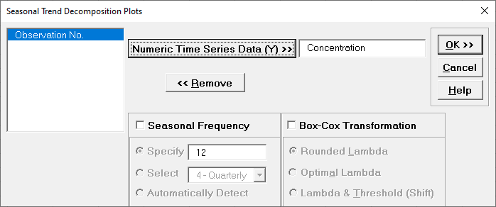
3. Click Concentration, click Numeric Time Series Data (Y) >>. Seasonal Frequency and Box-Cox Transformation should be unchecked as shown.

   
   
   

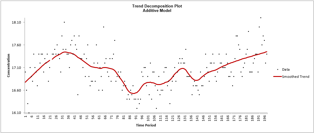
4. Click OK. A Trend Decomposition Plot for Concentration is produced.
   
   
   We can clearly see the wandering mean in this process. As discussed earlier, this can be modeled with exponential smoothing or with ARIMA after differencing.


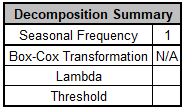
5. A Decomposition Summary report is also included to the right of the plot, indicating seasonal frequency and Box-Cox parameters (if applicable):
   
   
   Seasonal Frequency = 1 denotes a nonseasonal process.
   
   
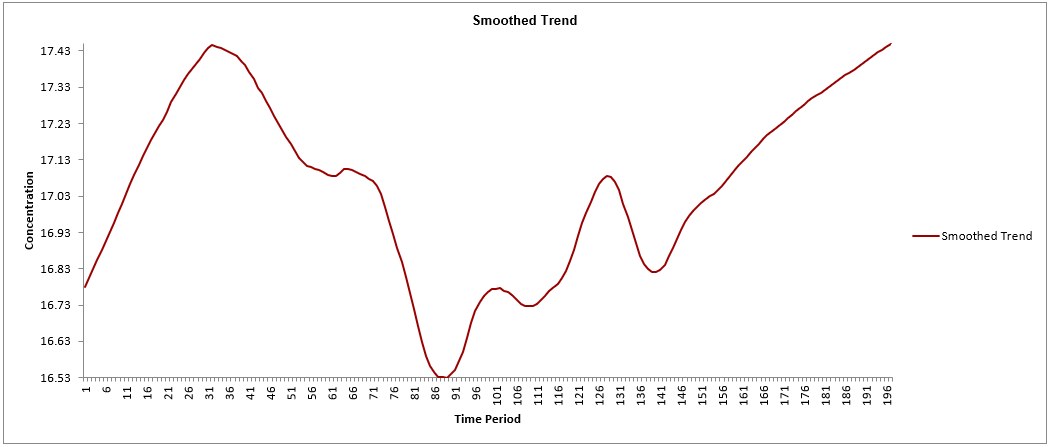
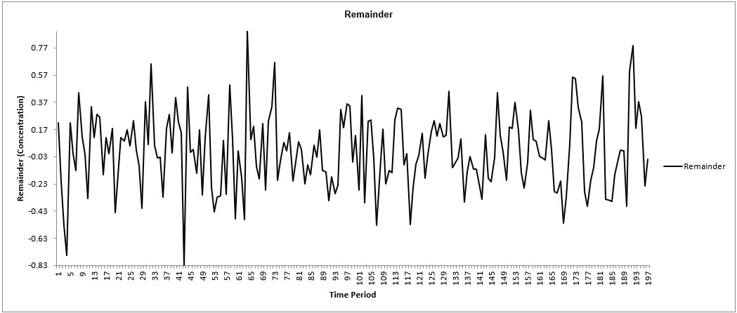
6. The Smoothed Trend and Remainder Plots are also produced as shown:
   
   
   
   

   Monthly Airline Passengers - Series G

7. Open Monthly Airline Passengers - Series G.xlsx (Sheet 1 tab). This is the Series G data from Box and Jenkins, monthly total international airline passengers for January 1949 to December 1960.
   
   
8. Click SigmaXL > Time Series Forecasting > Seasonal Trend Decomposition Plots. Ensure that the entire data table is selected. If not, check Use Entire Data Table. Click Next.
   
   
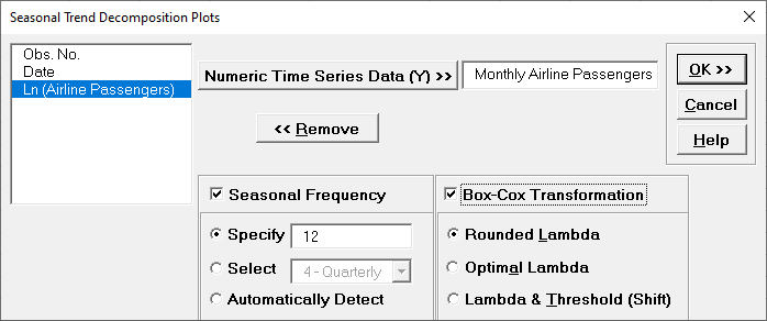
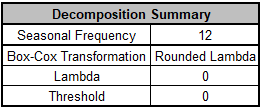
9. Select Monthly Airline Passengers, click Numeric Time Series Data (Y). Check Seasonal Frequency with Specify = 12. Check Box-Cox Transformation with Rounded Lambda (selected because the Run Chart showed an increase in the seasonal variance over time).
   
   
   Seasonal Frequency Specify also permits the entry of multiple frequencies.
   
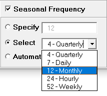
   Seasonal Frequency Select gives a drop-down list of commonly used seasonal frequencies:
   
   
   Seasonal Frequency Automatically Detect should be used if uncertain what the seasonal frequency value is (or do a Spectral.html prior to the Seasonal Trend Decomposition Plots).
   
   Box-Cox Transformation with Rounded Lambda will select Lambda = 0 (Ln), 0.5 (SQRT) or 1 (Untransformed). Threshold (Shift) is computed automatically if the time series data includes 0 or negative values, otherwise it is 0.
   
   Box-Cox Transformation with Optimal Lambda uses the range of 0 to 1 for Lambda. Threshold is computed automatically if the time series data includes 0 or negative values.
   
   Box-Cox Transformation with Lambda & Threshold (Shift) if left blank, will compute optimal lambda and threshold. The user may also specify Lambda and Threshold. Lambda may be specified outside of the 0 to 1 range, but practically for time series analysis, should be limited to -1 to 2. Threshold is typically 0, but if the time series data includes 0 or negative values, a negative threshold value should be entered that is smaller than the minimum data value. This value will be subtracted from the data resulting in positive time series values.
   
   
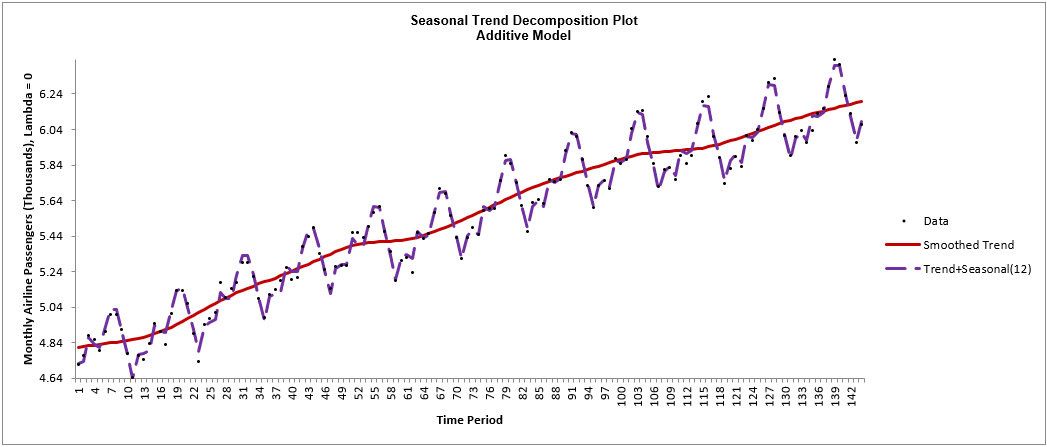
10. Click OK. A Seasonal Trend Decomposition Plot for Monthly Airline Passengers is produced.
    
    
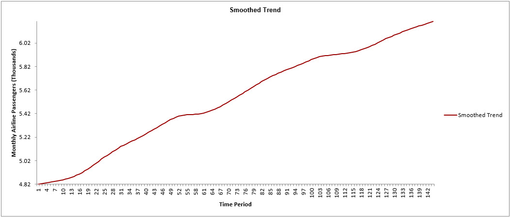
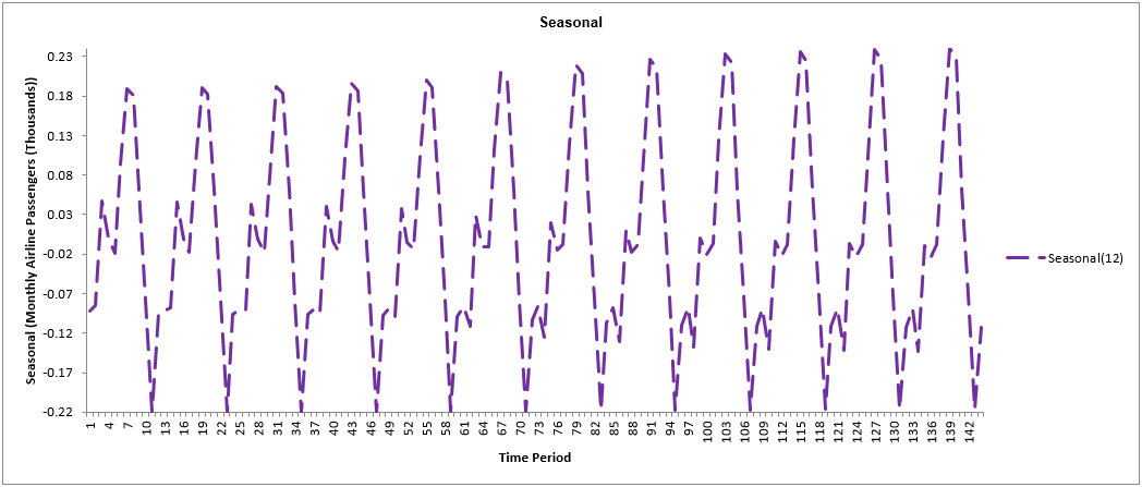
    Here we see a strong positive trend as well as the monthly seasonal effect. Note that this is the Lambda = 0 (Ln transformed) data. The Box-Cox transformation information is given in the Decomposition Summary report to the right of the plot:
    
    
    Seasonal Frequency is 12 and Lambda = 0. The Ln transformed data are displayed to maintain an additive model, which is easier to interpret than a multiplicative model.
    
    
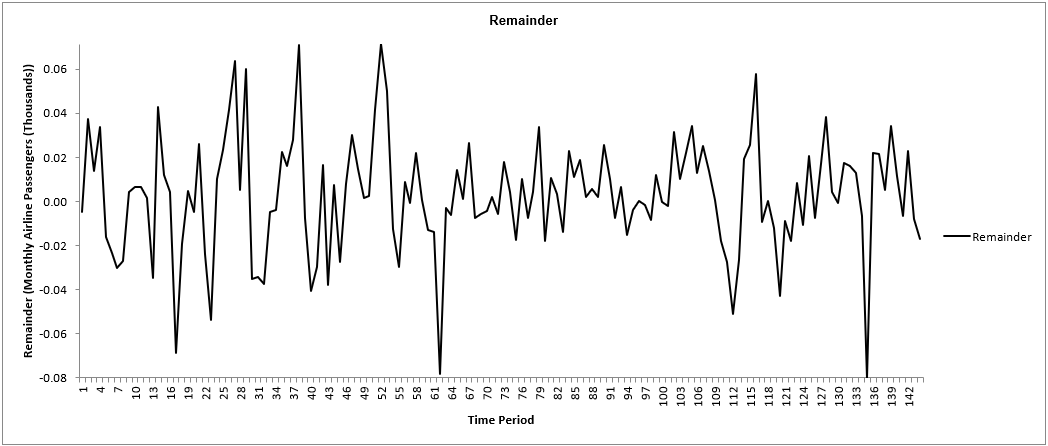
11. The Smoothed Trend, Seasonal and Remainder Plots are also produced as shown:
    
    
    
    
    
    
    

    Daily Electricity Demand with Predictors ElecDaily

12. Open Daily Electricity Demand with Predictors ElecDaily.xlsx (Sheet 1 tab). This is daily electricity demand (GW) for the state of Victoria, Australia, every day during 2014 (Hyndman, fpp2). This data has a seasonal frequency = 7 (observations per week).
    
    
13. Click SigmaXL > Time Series Forecasting > Seasonal Trend Decomposition Plots. Ensure that the entire data table is selected. If not, check Use Entire Data Table. Click Next.
    
    
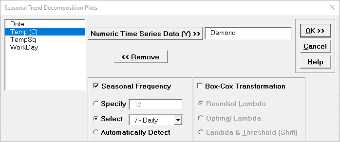
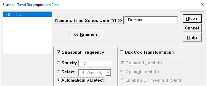
14. Select Demand, click Numeric Time Series Data (Y) >>. Check Seasonal Frequency with Select = 7-Daily selected from the drop-down list. Uncheck Box-Cox Transformation.
    
    
    
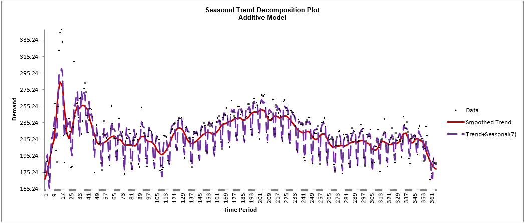
15. Click OK. A Seasonal Trend Decomposition Plot for Demand is produced.
    
    
    Here we see the daily seasonal effect. As discussed earlier, some of the trend patterns can be explained by the predictors Temp (C), TempSq and WorkDay.
    
    
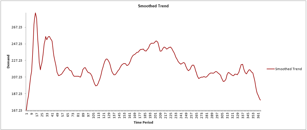
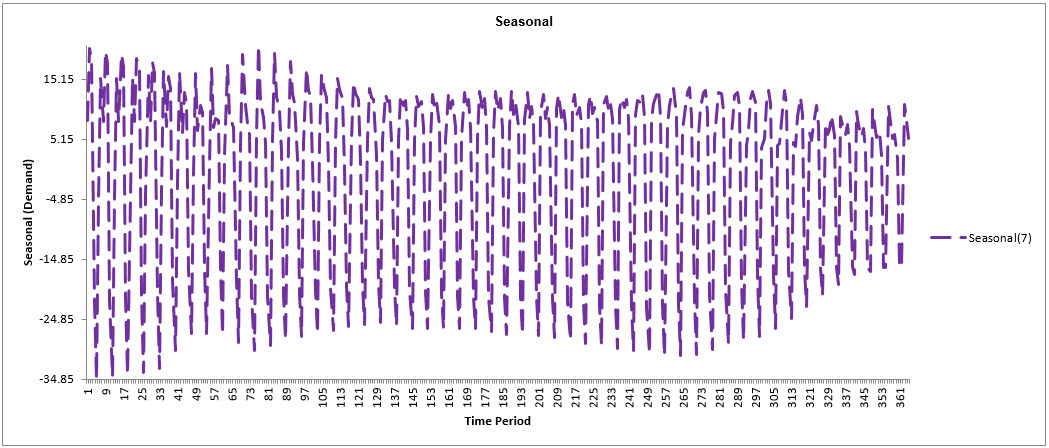
16. The Smoothed Trend, Seasonal and Remainder Plots are also produced as shown:
    
    
    
    
    
    
    

    Sales with Indicator - Modified Series M

17. Open Sales with Indicator - Modified Series M.xlsx. (Sheet 1 tab). This is modified Series M data from Box and Jenkins, with 50 quarters of corporate sales values along with a leading indicator. The data is treated as nonseasonal, as done in Box and Jenkins.
    
    
18. Click SigmaXL > Time Series Forecasting > Seasonal Trend Decomposition Plots. Ensure that the entire data table is selected. If not, check Use Entire Data Table. Click Next.
    
    
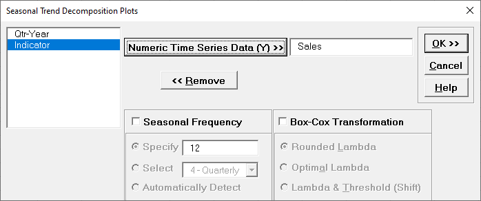
19. Select Sales, click Numeric Time Series Data (Y) >>. Seasonal Frequency and Box-Cox Transformation should be unchecked as shown.
    
    
    
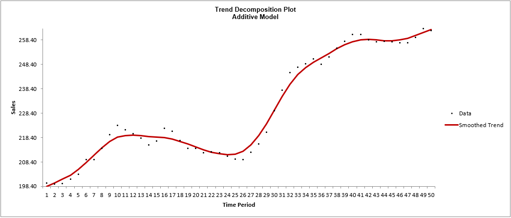
20. Click OK. A Trend Decomposition Plot for Concentration is produced.
    
    
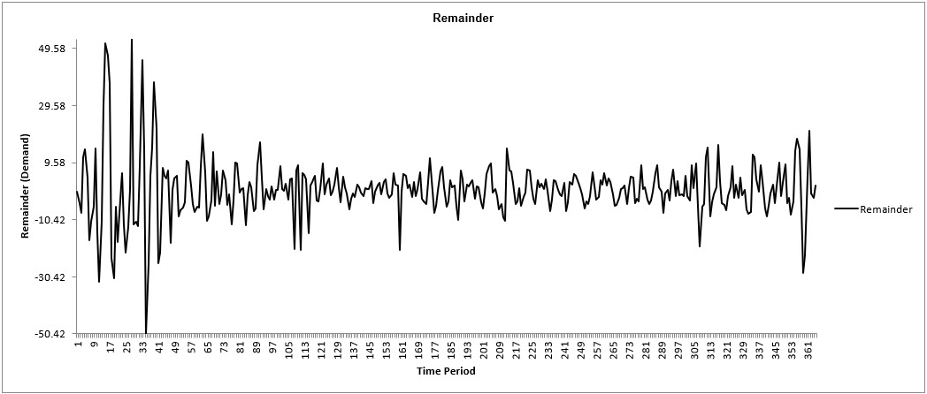
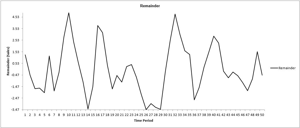
    Here we see an overall positive trend over the 50 quarters.
    
    
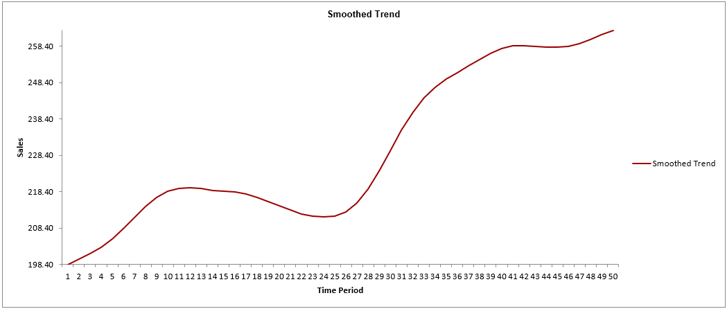
21. The Smoothed Trend and Remainder Plots are also produced as shown:
    
    
    
    
    

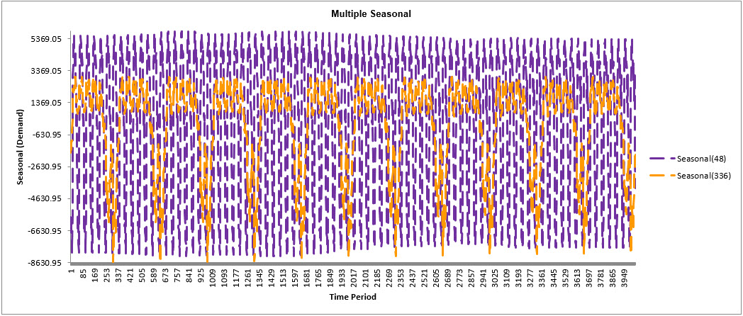
    Half-Hourly Multiple Seasonal Electricity Demand Taylor

22. Open Half-Hourly Multiple Seasonal Electricity Demand - Taylor.xlsx (Sheet 1 tab). This is halfhourly electricity demand (MW) in England and Wales from Monday, June 5, 2000 to Sunday, August 27, 2000 (taylor, R forecast). This data has multiple seasonality with frequency = 48 (observations per day) and 336 (observations per week), with a total of 4032 observations.
    
    
23. Click SigmaXL > Time Series Forecasting > Seasonal Trend Decomposition Plots. Ensure that the entire data table is selected. If not, check Use Entire Data Table. Click Next.
    
    
24. Select Demand, click Numeric Time Series Data (Y) >>. Seasonal Frequency with Automatically Detect. Uncheck Box-Cox Transformation.
    
    
    
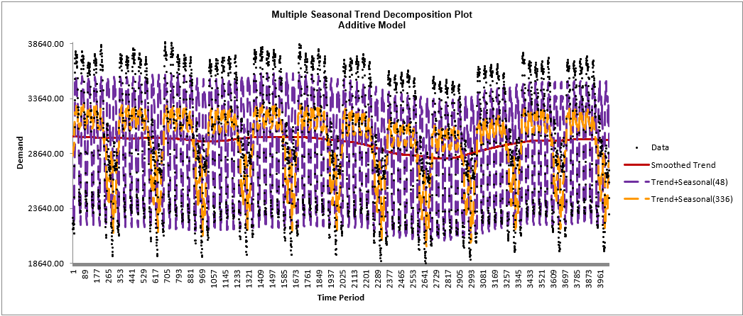
25. Click OK. A Seasonal Trend Decomposition Plot for Demand is produced.
    
    
    Automatic detection of seasonal frequency gives 48, 336, as obtained earlier with the Spectral.html. Here we see the half-hourly multiple seasonal effect with 48 observations per day and 336 observations per week.
    
    
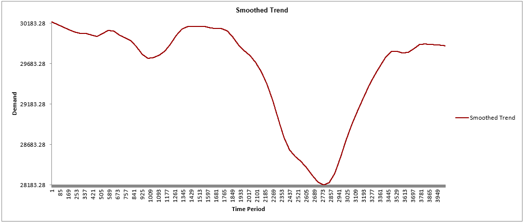
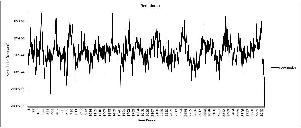
26. The Smoothed Trend, Seasonal and Remainder Plots are also produced as shown:
    
    
    
    
    
    
    

The Seasonal Trend Decomposition Plots are useful to visually distinguish trend and seasonal components in the time series data. If the Seasonal Frequency is unchecked, a Trend Decomposition Plot is produced as the first chart, showing the raw data and the trend. The trend component uses data smoothing, rather than a linear trend so that it may display either a linear trend or cyclical patterns. If a single seasonal frequency is specified, a Seasonal Trend Decomposition Plot is produced, showing the data, smoothed trend and seasonal component. If a multiple seasonal frequency is specified, a Multiple Seasonal Trend Decomposition Plot is produced, showing the data, smoothed trend and multiple seasonal component.

The second chart shows just the smoothed trend; the third chart (if applicable) shows just the seasonal or multiple seasonal component. The final chart is the remainder component.

This is an additive decomposition model, so the sum of the trend value + seasonal value(s) + remainder value gives the original data value. A multiplicative equivalent may be obtained by specifying the Box-Cox Transformation with Lambda = 0, which is a Ln transformation, but the charts will display the transformed data to maintain an additive model. Rounded or Optimal Lambda may also be used, but will only consider the range of values 0 to 1 (this conservative approach is used in time series forecasting, unlike regular Box-Cox in SigmaXL which uses a range of -5 to 5). See Appendix: Box-Cox Transformation.

The decomposition algorithms used here are the same as used in Exponential Smoothing Multiple Seasonal Decomposition (MSD), and ARIMA MSD. The seasonal component is first removed through decomposition, a nonseasonal exponential smooth model fitted to the remainder + trend, and then the seasonal component is added back in. This is mainly used for high seasonal frequency and/or multiple seasonal frequency time series. For further details and formulas, see Appendix: Seasonal Trend Decomposition.