Optimal Analyze
- Home /
- Optimal Analyze

Optimal design of experiments is a method for planning experiments to maximize the amount of information gained while using the fewest resources. The design of experiments is undertaken by an iterative search algorithm that seeks to optimize a design criterion for a given model with a specified number of runs. A total of 19 continuous/categorical factors are permitted (maximum of 10 categorical with up to 10 levels). Linear constraints may be specified for the continuous factors.
In SigmaXL, MIDACO Solver (Mixed Integer Distributed Ant Colony Optimization) is used to solve the design criterion as an objective function. All continuous factors are coded as -1 to +1 and categorical factors and blocks are coded -1/0/1. The factors are solved as a vector with a maximum size of 3000 values. This vector is then reshaped as an nxk matrix to solve the objective function value. This approach is competitive with the coordinate exchange algorithm and in some cases superior to it. The disadvantage is that it can be slow for large models (see below for MIDACO settings) and with 19 continuous factors, is limited to 157 runs.
A candidate matrix is automatically created using a 5-level grid with coded values: -1, -0.5, 0, +0.5, +1, for up to 8 continuous factors; 3-level for 9 to 12 continuous factors and 2-level with center point for 13 to 19 continuous factors. The solved continuous values are mapped to the candidate matrix using minimum sum-of-squares distance for each row.
If there are no linear constraints specified, the mapped values are then used as starting values for MIDACO to solve the objective function as a combinatorial problem, selecting runs from the candidate matrix, resulting in a design solution that has at most 5 levels for each factor. While this yields a solution that is not as optimal as one where the factor values can take on any value between -1 to +1, this makes the implementation of the actual experiment easier for the practitioner.
If Continuous Linear Constraints is checked and linear constraints are specified, the above step is skipped and continuous factors in the design will include coded values from -1 to +1 that satisfy the constraint formula(s). If no constraint formula is specifed, the above step is skipped and continuous factors in the design will include coded values from -1 to +1.
Note that for analysis, constraint formulas will automatically be applied to Optimize and Multiple Response Optimization, but not to Contour and Surface Plots.The Number of Additional Runs/Points for Modelspecify the number of runs in addition to the minimum required by the model (i.e., number of coefficient terms including constant). The default value is 6. If 0 is specified (with Minimum Number of Replicate Runs/Points = 0 and Minimum Number of Center Points for Continuous = 0), the error df will be 0; the recommended minimum additional runs is 3.
IfMinimum Number of Replicate Runs/Points > 0or Minimum Number of Center Points for Continuous > 0, a constraint is added to the objective function to ensure that these requirements are met. Note that i Minimum Number of Center Points for Continuous = 0),and there are categorical factors, the categorical factor levels will not necessarily be balanced.
The Total No. of Runs = Number of runs required by the model + Number of Additional Runs/Points for Model + Minimum Number of Replicate Runs/Points + Minimum Number of Center Points for Continuous
The MIDACO settings of Maximum Time (seconds) and Maximum Function Evaluations with no Change (x1000) may be modified. The default settings are 300 seconds and 100,000 function evaluations, but 600 seconds and 1,000,000 evaluations may be needed for a complex problem with more than 30 terms, includes multi-level categorical terms or constraints.
A D-Optimal design maximizes the determinant of the XX'XX information matrix, which minimizes the volume of the joint confidence region of the estimated regression coefficients. This results in good overall model precision, so is recommended as a general purpose alternative to screening and two-level factorial designs.
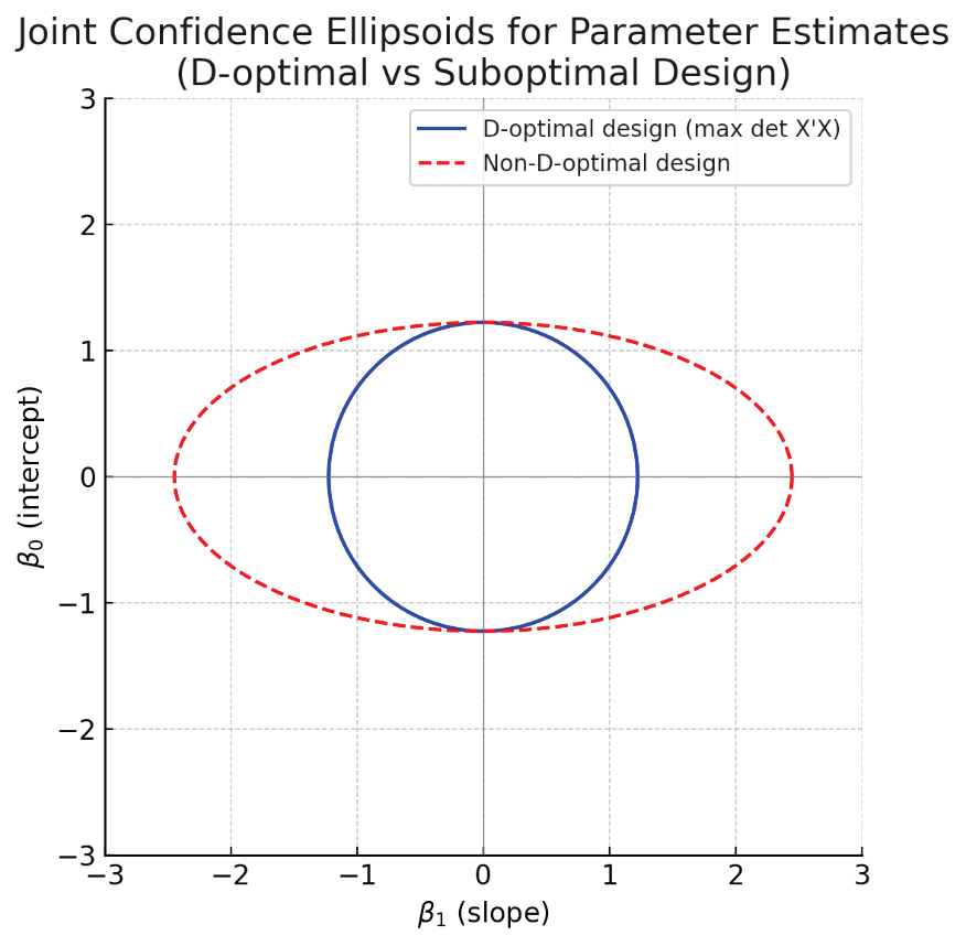
Joint confidence ellipsoids (95% confidence) for two regression parameters (β0 and β1) under two different experimental designs. The D-optimal design (blue ellipse) leads to a much smaller ellipse (lower joint uncertainty) than a suboptimal design (red ellipse) that has a lower det (XX'XX). In higher dimensions, D-optimality analogously minimizes the hyper-volume of the confidence ellipsoid for all parameters.
This property makes D-optimal designs especially useful when we care about the overall precision of all model coefficients together, rather than any single coefficient in isolation.
An A-Optimal design minimizes the trace of (XX'XX)-1 (the trace of the inverse of the information matrix), which minimizes the average variance of the estimated regression coefficient terms and is recommended for screening designs by Jones. et. al. [4].
An I-Optimal design minimizes the trace of (XX'XX)-1MM, where MM is the moment matrix for the given model. This minimizes the average prediction variance (integrated variance) over the design space, which can be thought of as minimizing the area under the Fraction of Design Space (FDS) Plot. Since the primary objective of a Response Surface design is accurate prediction and optimization, I-Optimality is recommended for RSM designs. For details on the moment matrix, see Goos and Jones [1]. Note that currently I-Optimal is not available if there are linear constraints.
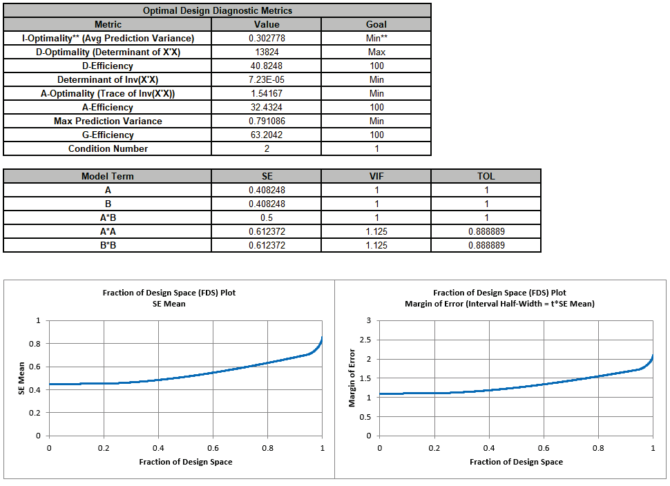
Optimal Design Diagnostic Metrics
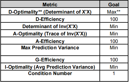
The double asterisks ** denotes the metric that is used as the objective function for MIDACO. The goal is given as Max, Min or numeric value. For formula details see the Appendix: Optimal Design.
The D, A and G-Efficiency metrics compare the efficiency of the design to that of an ideal orthogonal design in terms of the respective optimality criterion. A full or fractional factorial design (without center points) would have D-Efficiency, A-Efficiency and G-Efficiency all equal to 100%.
The efficiency metrics are easier to interpret than the optimality metrics since they are scaled from 0 to 100, but note that for D and A-Efficiency, we do not have “rules of thumb” to aid in interpretation. These efficiency metrics should be used as indicators to compare designs that have the same number of runs [1].
Max Prediction Variance and G-Efficiency are calculated using Monte Carlo sampling of the design space as done in the Fraction of Design Space (FDS) Plot with 1e6 replicates. Therefore, calculations for the same design might vary slightly. Montgomery et al. [6] note: “Usually a G-Efficiency of around 50% or higher is desired. Standard response surface designs in regularly shaped regions typically have G-Efficiencies well above 50%, and often they are in the 70-90% range."
Montgomery et al. [7] give a rule of thumb for condition number: > 100 indicates moderate multicollinearity.
Model term SE, VIF and TOL are also reported. These are the same values that would be
obtained in a regression
model with error standard deviation = 1.
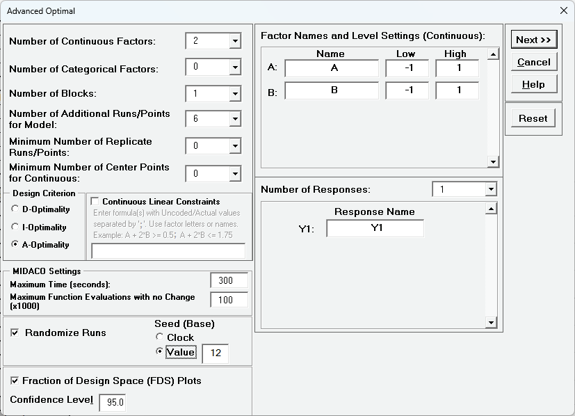
Now we will evaluate and compare Optimal designs for 2 Continuous Factors. Click SigmaXL > Design of Experiments > Advanced Design of Experiments: Optimal > Optimal Designs Select Design Criterion as D-Optimality, Select Seed (Base) Value = 12 and other default options as shown:

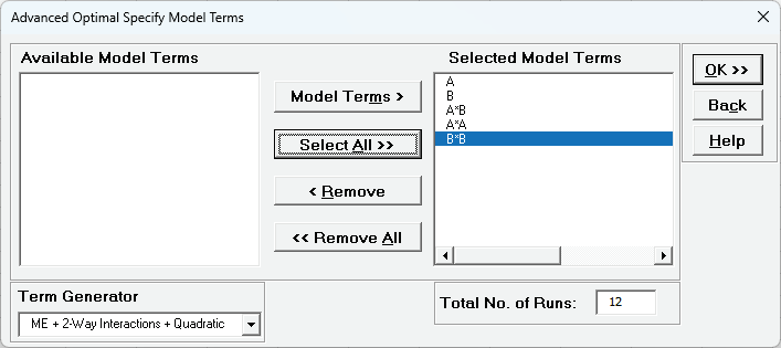
Click Next>> to specify the model to be used in the D-Optimal design:

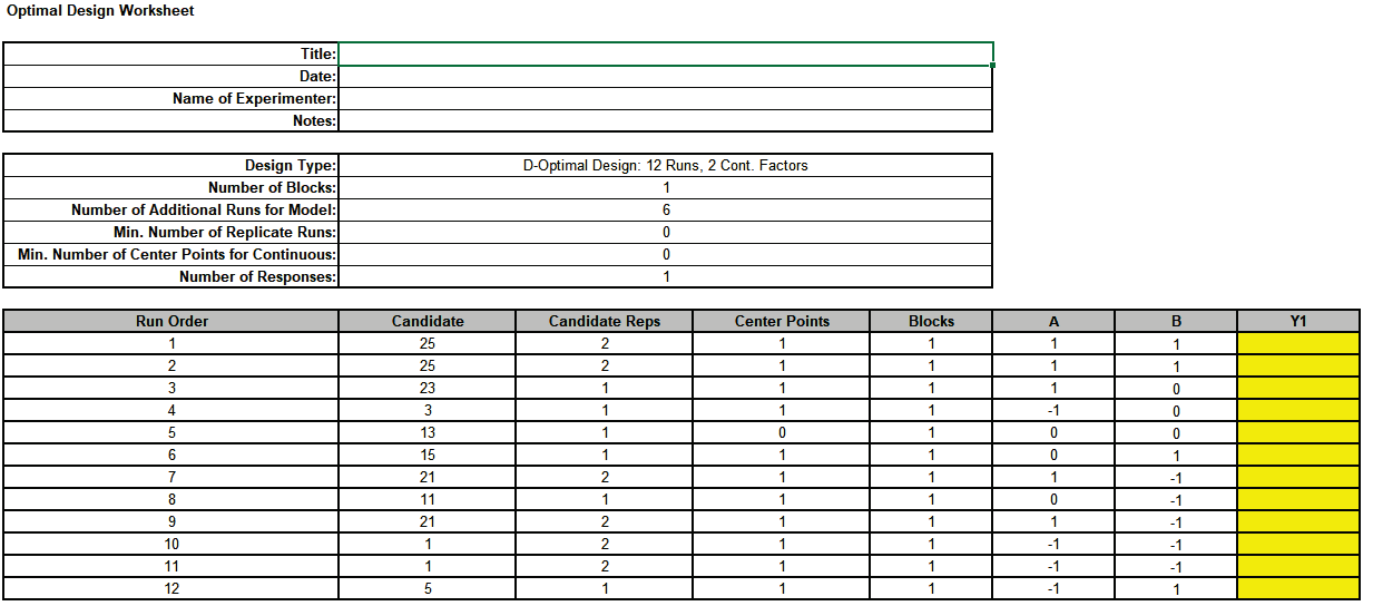
. This is a 2 Factor, D-Optimal design with a Main Effects + 2-Way Interactions + Quadratic model, with 6 additional runs for model, giving a Total No. of Runs = 12 The FDS Plot uses the same model as the D-Optimal design with Confidence Level = 95%. FDS will also use the Fixed Seed = 12 for replicable results. Click OK.
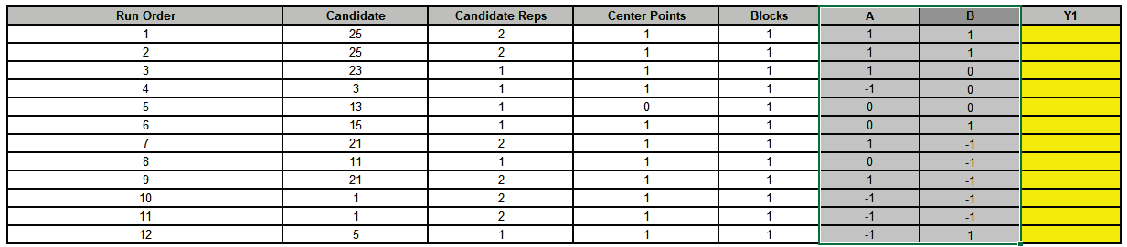
The Design Worksheet, Optimal Design Diagnostic Metrics, Model Term SE and VIF, and FDS Plots are given.
These will be compared and discussed after all 3 designs are produced.
Since we have only two continuous factors, we can visualize the design using a Scatter Plot of the factor settings and use Candidate Reps as data labels. Note that this is an optional step and would not typically be a part of the design process, but is useful for understanding how the different optimality criterion affect the factor level settings. Select factor columns A and B as shown:
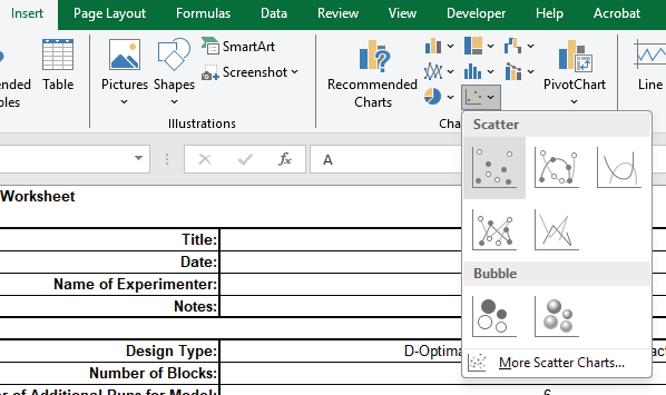
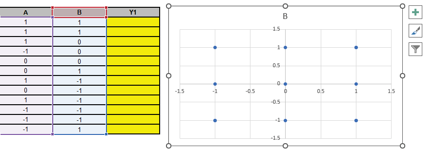
Click Excel > Insert t and select Scatter Charts as shown. Factor A will be the X axis, Factor B the Y Axis:
Drag the Scatter Chart adjacent to the Y1 response column
With the chart selected, click + and check Axis Titles:
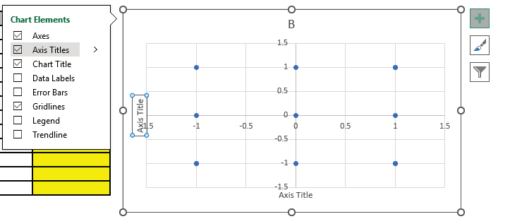
Modify the Chart Title and Axis Titles as shown
With the chart selected, click + , check Data Labels and select More Options:
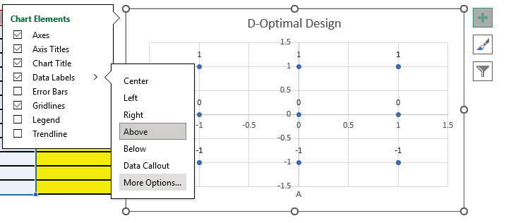
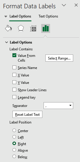
Check Label Contains - Value From Cells. Uncheck other Label Options. Select Label Position Right:
For Data Label Range, select Candidate Reps D16 to D27 as shown.
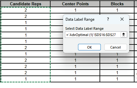
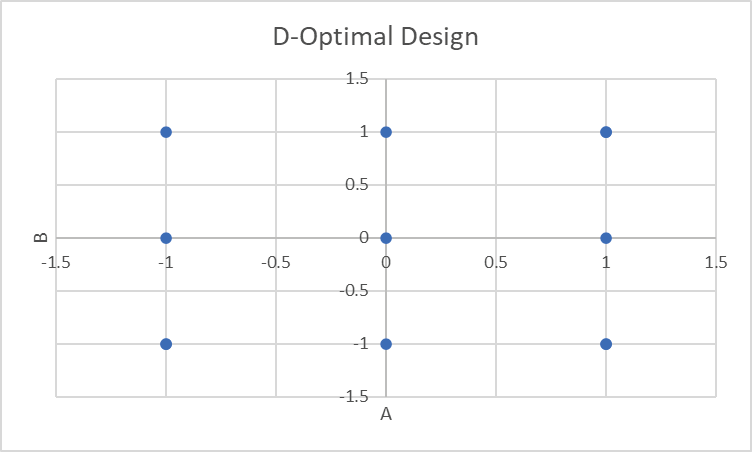
Click OK. Close Format Data Labels dialog. The final Scatter Chart is shown:
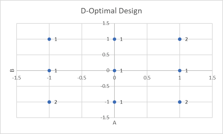
From this chart of factor settings for A, B, we can see that the D-Optimal design has selected a 3-level full-factorial and added replicates in the corners.
Now we will repeat steps 1 to 3 using I-Optimality. Click SigmaXL > Design of Experiments > Advanced Design of Experiments: Optimal > Optimal Designs. Select Design Criterion as I-Optimality, select Seed (Base) Value = 12 and other default options as shown:

Click Next>> to specify the model to be used in the I-Optimal design:
This is a 2 Factor, I-Optimal design with a Main Effects + 2-Way Interactions + Quadratic model, with 6 additional runs for model, giving a Total No. of Runs = 12. The FDS Plot uses the same model as the I-Optimal design with Confidence Level = 95%. FDS will also use the Fixed Seed = 12 for replicable results. Click OK.
The Design Worksheet, Optimal Design Diagnostic Metrics, Model Term SE and VIF, and FDS Plots are given.

These will be compared and discussed after all 3 designs are produced.
Repeat steps 5 to 13 to create a Scatter Chart of Factor Settings:
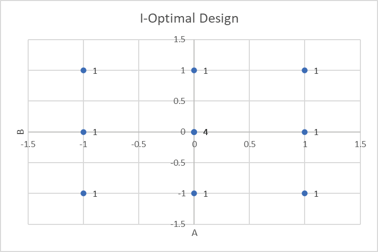
From this chart of factor settings for A, B, we can see that the I-Optimal design has also selected a 3-level full-factorial and added replicates to the center points.
Now we will repeat steps 1 to 3 using A-Optimality. Click SigmaXL > Design of Experiments > Advanced Design of Experiments: Optimal > Optimal Designs. Select Design Criterion as A-Optimality, select Seed (Base) Value = 12 and other default options as shown:
Click Next>> to specify the model to be used in the A-Optimal design: OK.

This is a 2 Factor, A-Optimal design with a Main Effects + 2-Way Interactions + Quadratic model, with 6 additional runs for model, giving a Total No. of Runs = 12 The FDS Plot uses the same model as the A-Optimal design with Confidence Level = 95%. FDS will also use the Fixed Seed = 12 for replicable results. Click OK.
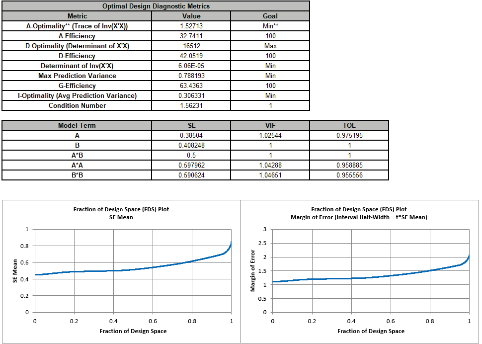
The Design Worksheet, Optimal Design Diagnostic Metrics, Model Term SE and VIF, and FDS Plots are given.

Repeat steps 5 to 13 to create a Scatter Chart of Factor Settings:
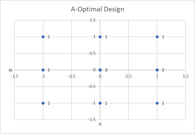
From this chart of factor settings for A, B, we can see that the A-Optimal design has also selected a 3-level full-factorial and added replicates to the center points and an edge point.
Next, we will create an Overly FDS Plot for the 3 designs. Click SigmaXL > Design of Experiments > Advanced Design of Experiments: Overlay FDS Plots. Select FDS Plot Sheets and enter Legend names as shown:
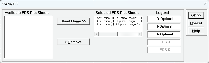
Clik Ok.
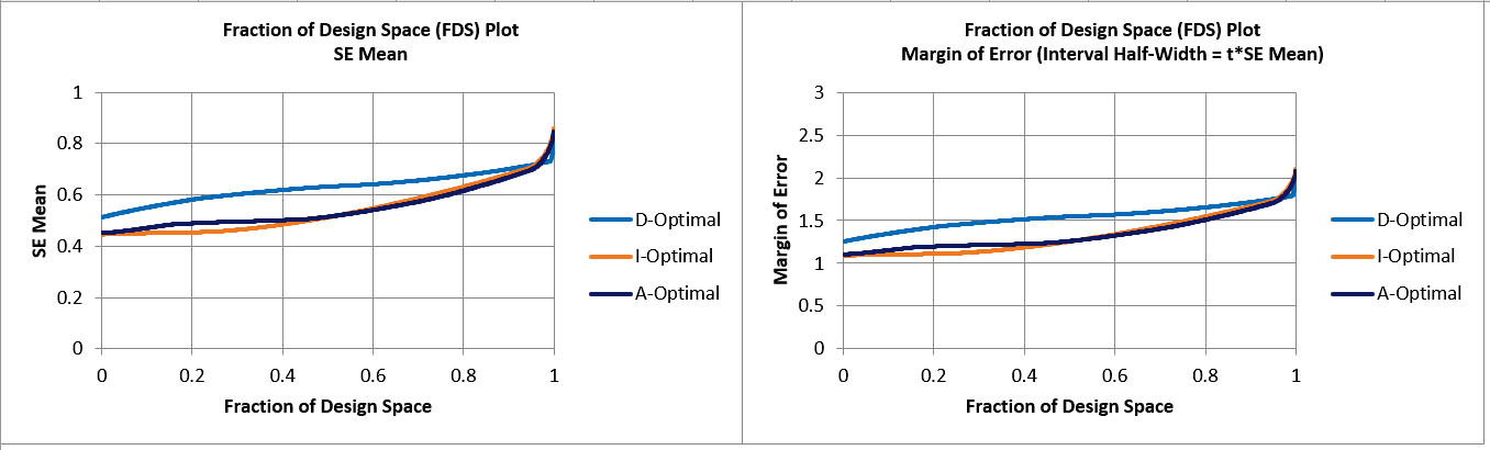
As expected, I-Optimal has the lowest overall SE Mean and Margin of Error since its optimality criterion minimizes average prediction error, but only slightly, and A-Optimal is approximately the same as I-Optimal for 50% of the design space.
D-Optimal has the largest SE Mean and Margin of Error except for a small percent of the design space (at the corners).
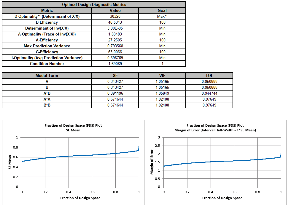
Now we will compare the Optimal Design Diagnostic Metrics for the 3 designs:
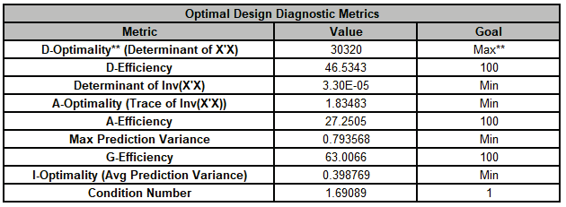
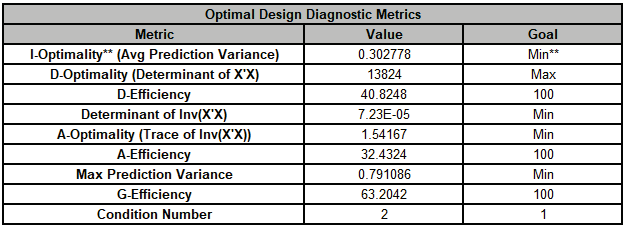
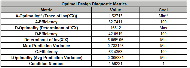
As expected, the Efficiency scores are highest for their respective optimality criterion. However, A-Optimality has the highest G Efficiency (i.e., lowest maximum variance), lowest Condition Number, approximately the same Avg Prediction Variance as I-Optimality, and a higher D Efficiency than the I-Optimal design.
The Model Term SE/VIF for D-Optimal are:
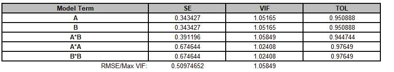
Note, RMSE has been added using the formula =SQRT(SUMSQ(C43:C47)/5). Max VIF is also shown.
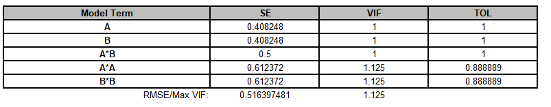
I-Optimal:
A-Optimal:
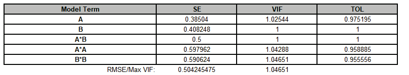
As expected, A-Optimal has the lowest RMSE for the Model Terms. It also has the lowest Max VIF score.
In conclusion, the best overall design choice amongst these 3 for this specific number of runs and model, is A-Optimal. Note that one cannot conclude that A-Optimal is generally preferred for a two factor RSM design, one would need to compare and evaluate for each design case. We will not consider analysis of response data with these designs here.
This example demonstrates the use of a D-Optimal design with constraints, as given in the paper by Montgomery D.C. et al. (2002) “Experimental Designs for Constrained Regions”, Quality Engineering, 14(4), pp. 587-601.
"An experimenter is investigating the bond strength of a particular adhesive. The adhesive is applied to two parts and then the assembly cured at an elevated temperature. The two factors of interest are the amount of adhesive applied (A) and the cure temperature (B). Over the ranges of these factors, taken from -1 to 1 on the usual coded design variable scale, the experimenter knows that if too little adhesive is applied and the cure temperature is too low, the parts will not bond satisfactorily… Furthermore, if the temperature is too high and too much adhesive is applied, either the parts will be damaged by stress or an inadequate bond will result."
The linear constraint formulas are given as:
A+B >= -0.5
A+B <= 1
The expected range of bond strength values is approximately 1 to 4. For demonstration purposes we will assume a process historical standard deviation = 0.1.
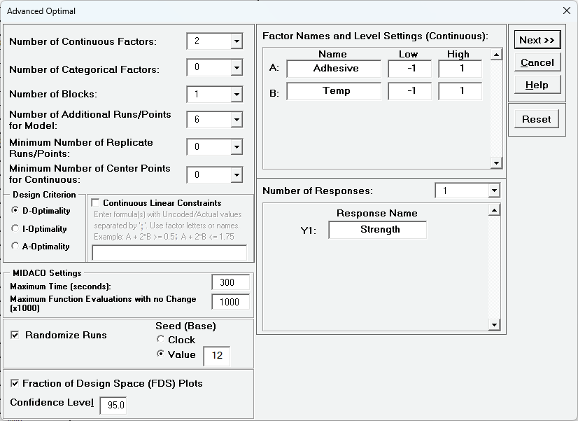
Click SigmaXL > Design of Experiments > Advanced Design of Experiments: Optimal > Optimal Designs. Use the default Number of Additional Runs/Points for Model = 6, Select Design Criterion as D-Optimality, MIDACO Settings - Maximum Function Evaluations with no Change (x1000) = 1000 0 (recommended for designs with constraints), select Seed (Base) Value = 12 enter Factor Names and Response Name as shown:
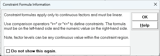
Check Continuous Linear Constraints. A message dialog appears with important information on constraint formulas:
Check OK. Enter the constraint formulas using factor letters: A+B <= 1; A+B>= -0.5
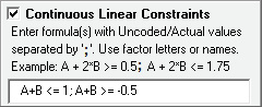
The semicolon is used as a separator for the constraint formulas. A comma is not permitted as that is reserved for an international decimal place.
Tips: letters are used for convenience and brevity. These will be displayed as factor names.
Carefully review that the constraint formulas are correct. Click Next >>
Select the Model Terms as shown for a ME + 2-Way Interactions + Quadratic RSM model as given in the paper:
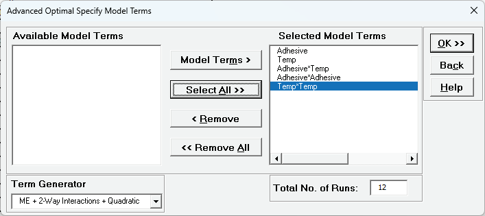
Check OK. This will take about one minute due to the revised MIDACO setting.
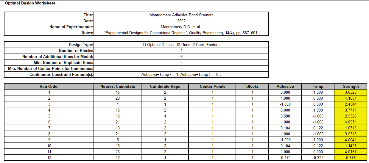
The Design Worksheet, Constraint Formulas, Optimal Design Diagnostic Metrics and Model Term SE/VIF are given as:
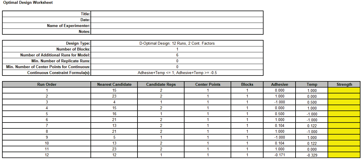
Note that with a constrained design, the continuous factors can take on any value between -1 and 1 (or low to high) and are displayed to 3 decimal places. The constraints can be checked by summing the two factor columns row-wise, but we will not do so here. The Continuous Constraint Formulas are given using factor names even though they were originally specified using factor letters.
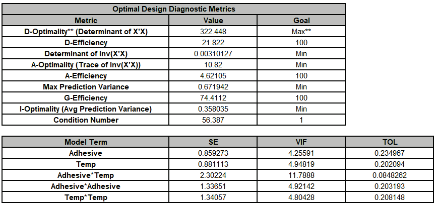
The D-Efficiency and A-Efficiency values are low but they cannot be used as a measure of design quality standalone, they are used for comparison to other designs as we did in Example 6. On the other hand, we see that the G-Efficiency is good and is greater than 50% as recommended by Montgomery. The condition number = 56.4 is high, but still less than Montgomery’s rule of thumb where > 100 is moderate. The maximum VIF score is 11.8 which is higher than the recommended maximum of 5, but this degree of multicollinearity is an unavoidable consequence of adding constraints to the design.
The FDS Plots and report are given as:
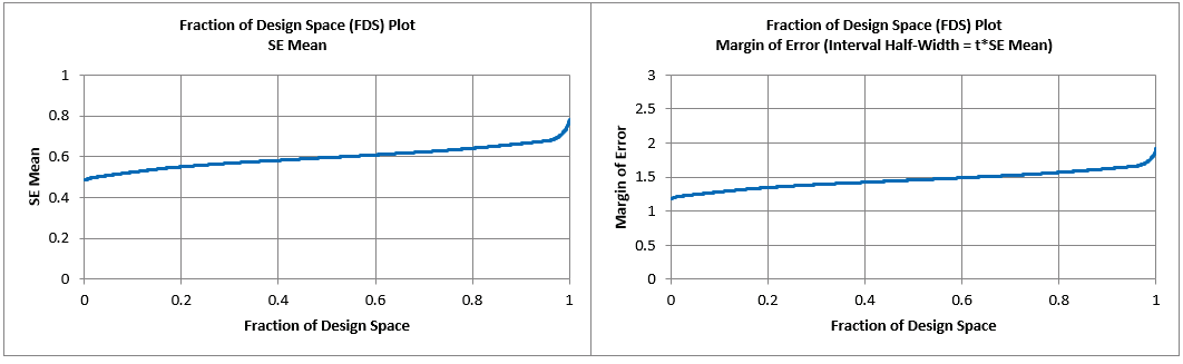
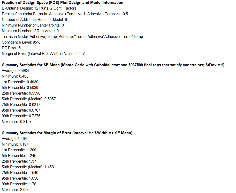
Looking at the 95th Percentile (i.e., 95% of the design space), we see that the SE Mean can be as large as 0.68 and the Margin of Error (Interval Half-Width) as large as 1.78.
To obtain units of Bond Strength, we multiply by the process historical standard deviation: SE Mean = 0.68*0.1 = 0.068 and Half-Width = 1.78*0.1 = 0.178. This is an acceptable margin of error for the bond strength which has an expected range of values of 1 to 4.
Note that the Confidence Level of 95% applies to the Margin of Error. The 95th Percentile applies to the Fraction/Proportion of Design Space.
Now we will create an Excel Scatter Chart of the factor settings. Repeat steps 5 to 13 in Example 6. Since Adhesive is the first column it is the X axis and Temp is the Y axis. The title is modified as shown. Candidate Reps are shown as data labels.
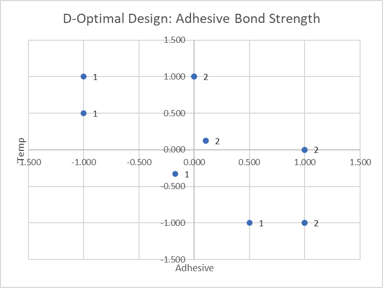
Notice that the constraints effectively remove two corners of the original square region of operability, and this results in an irregular experimental region. We can see that the constraint formulas have been met and that there are two replicates in the center of the constrained region, and at (0,1), (1,0), and (1,-1). Note that the center of the constrained region is not the same as (0,0) center points. If we wanted to ensure actual center points, we could have specified Min. Number of Center Points for Continuous > 0.
Open the file Montgomery Adhesive Bond Strength.xlsx. This has the design worksheet populated with Bond Strength values.
Click SigmaXL > Design of Experiments > Advanced Design of Experiments: Optimal > Analyze Optimal Design.
. Select Responses and Model Terms as shown with Term Generator as ME + 2-Way Interactions + Quadratic. This is the same model that was specified in the D-Optimal design. Residual Plots are checked. We will not modify Advanced Options.
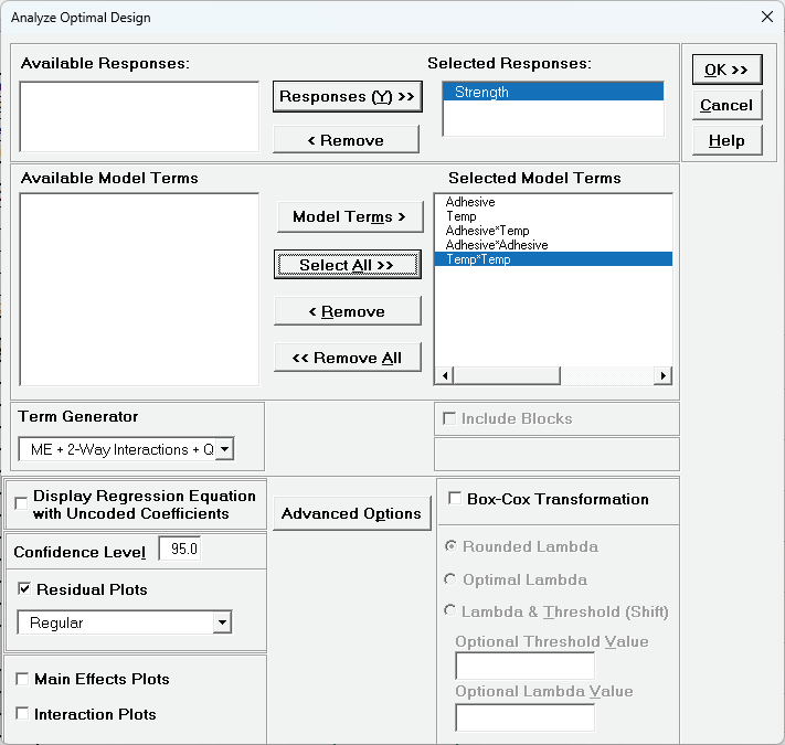
Note that for the analysis, constraint formulas will automatically be applied to Optimize, but not to Contour and Surface Plots.
Click OK.
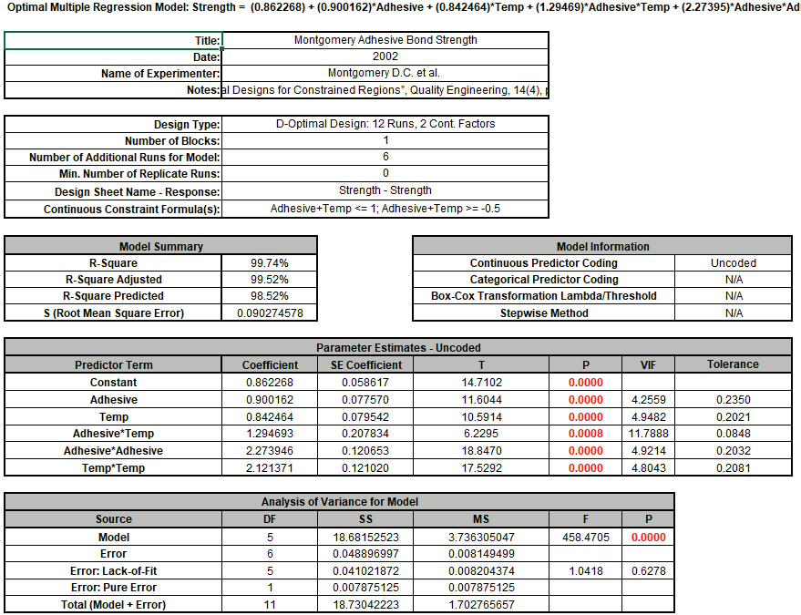
There is no significant Lack of Fit, all model terms are significant, and the R-Square, R-Square Adjusted and R-Square Predicted are very high. Note that the VIF and Tolerance values match those given in the design report, with the maximum VIF = 11.8 due to the design constraints. The Predictor Term SE Coefficient values divided by S match those given in the design report.
Click on the AdvOpt - Residuals Strength Sheet
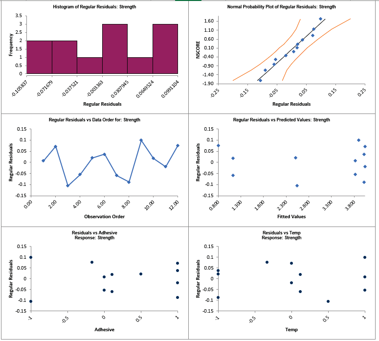
The residuals look good with no obvious non-normality or patterns.
Click on the Sheet AdvOpt - Model Strength. Scroll to the Predicted Response Calculator. Enter Adhesive = 0, Temp = 0 to predict Strength with the 95% confidence interval for the long term mean and 95% prediction interval for individual values:

The Margin of Error (Interval Half-Width) is 1.006 - 0.862 = 0.144, which is close to what we estimated using the FDS Plot. Given that the Strength range of values is approximately 1 to 4, this is an acceptable margin of error for prediction.
Note that the Predicted Response Calculator allows settings that are outside of the constraint region, in which case the predicted response would be an extrapolation.
Next, we will use SigmaXL's built in Optimizer. Scroll to view the Optimize Options:
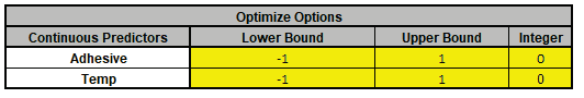
Here we can constrain the lower and upper bounds of the continuous predictors, but we will leave the default settings as is. Note that the constraints: Adhesive+Temp <= 1; Adhesive+Temp>= -0.5 are automatically applied in the optimization.
Scroll back to view the Goal setting and Optimize button. Specify Goal = Maximize.
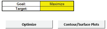
The optimizer uses MIDACO to solve for the desired response goal that satisfies the constraint formulas and will require about 1 minute to solve.
Click Optimize. The response solution and prompt to paste values into the Input Settings of the Predicted Response Calculator is given:
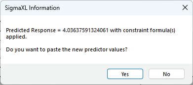
Click Yes to paste the values.

So Adhesive = 1 and Temp = 0 give maximum Bond Strength. This agrees with the maximum settings given in the paper, although other maximum values are also possible.
Next, we will create a Contour/Surface Plot to view those alternative settings. Click the Contour/Surface Plots button
A new sheet is created, AdvAug1 - Contour that displays the plots:
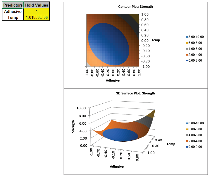
. The Contour and Surface Plots do not show the constraint region, but constraint lines (using points from the Scatter Chart) can be manually drawn on the contour plot as shown (with Contour Plot enlarged):
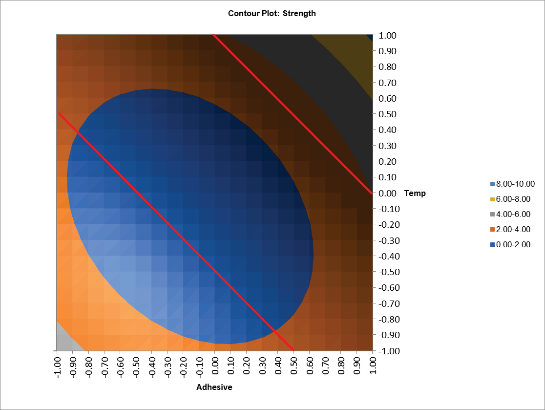
Note that the strength values outside of the constraint regions are extrapolated.
We can see that, in addition to Adhesive = 1, Temp = 0 as given by the Optimizer, other settings that maximize bond strength and satisfy the constraints are: Adhesive = -1, Temp = 1; Adhesive = 1, Temp = -1 and Adhesive = 0, Temp = 1. These settings can be entered in the predicted response calculator to obtain a predicted response with confidence intervals.
Given the possible multiple solutions, a cost response could be added and multiple response optimization (MRO) used to provide a (likely) unique solution. MRO also automatically applies the constraint formulas.


