One Sample t-Test

How Do I Perform Power and Sample Size Calculations for a One Sample t-Test?

Power and Sample Size One Sample t-Test Customer Data

Using the One Sample t-Test, we determined that Customer Types 1 and 3 resulted in Fail to reject H0: μ=3.5. A failure to reject H0 does not mean that we have proven the null to be true. The question that we want to consider here is What was the power of the test? Restated, What was the likelihood that given Ha: μ≠3.5 was true, we would have rejected H0 and accepted Ha? To answer this, we will use the Power and Sample Size Calculator.

Tip: Typical sample size rules of thumb address confidence interval size and robustness to normality (e.g. n=30). Computing power is more difficult because it involves the magnitude of change in mean to be detected, so one needs to use the power and sample size calculator.

Please use the following guidelines when using the power and sample size calculator:

Power >= .99 (Beta Risk is <= .01) is considered Very High Power

Power >= .95 and < .99 (Beta Risk is <=.05) is High Power

Power >= .8 and < .95 (Beta Risk is <=.2) is Medium Power. Typically, a power value of .9 to detect a difference of 1 standard deviation is considered adequate for most applications. If the data collection is difficult and/or expensive, then .8 might be used.

Power >= .5 and < .8 (Beta Risk is <=.5) is Low Power not recommended.

Power < .5 (Beta Risk is> .5) is Very Low Power do not use!

1. Click SigmaXL > Statistical Tools > Power and Sample Size Calculators > 1 Sample t-Test Calculator. We will only consider the statistics from Customer Type 3 here. We will treat the problem as a two sided test with Ha: Not Equal To to be consistent with the original test.


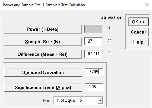
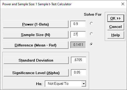
2. Enter 27 in Sample Size (N). The difference to be detected in this case would be the difference between the sample mean and the hypothesized value i.e. 3.6411 3.5 = 0.1411. Enter 0.1411 in Difference. Leave Power value blank, with Solve For Power selected (default). Given any two values of Power, Sample size, and Difference, SigmaXL will solve for the remaining selected third value. Enter the sample standard deviation value of 0.6705 in Standard Deviation. Keep Alpha and Ha at the default values as shown:
   
   
   
   
3. Click OK. The resulting report is shown:






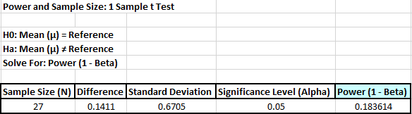
4. A power value of 0.1836 is very poor. It is the probability of detecting the specified difference. Alternatively, the associated Beta risk is 1-0.1836 = 0.8164 which is the probability of failure to detect such a difference. Typically, we would like to see Power > 0.9 or Beta < 0.1. In order to detect a difference this small we would need to increase the sample size. We could also set the difference to be detected as a larger value.


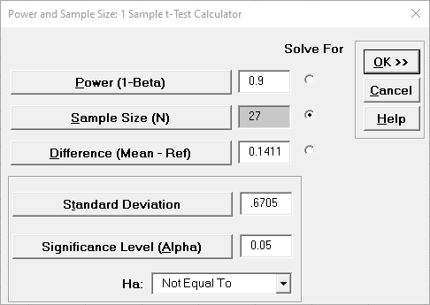
5. First we will determine what sample size would be required in order to obtain a Power value of 0.9. Click Recall SigmaXL Dialog menu or press F3 to Recall Last Dialog. Select the Solve For Sample Size button as shown. It is not necessary to delete the entered sample size of 27 it will be ignored. Enter a Power Value of .9:
   
   
   
   
6. Click OK. The resulting report is shown:
   
   
   
   
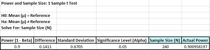
7. A sample size of 240 would be required to obtain a power value of 0.9. The actual power is rarely the same as the desired power due to the restriction that the sample size must be an integer. The actual power will always be greater than or equal to the desired power.
   
   
8. Now we will determine what the difference would have to be to obtain a Power value of 0.9, given the original sample size of 27. Click Recall SigmaXL Dialog menu or press F3 to Recall Last Dialog. Select the Solve For Difference button as shown:
   
   
   
   
9. Click OK. The resulting report is shown:
   
   
   
   
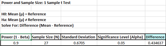
10. A difference of 0.435 would be required to obtain a Power value of 0.9, given the sample size of 27.
    

Power and Sample Size One Sample t-Test Graphing the Relationships between Power, Sample Size, and Difference

In order to provide a graphical view of the relationship between Power, Sample Size, and Difference, SigmaXL provides a tool called Power and Sample Size with Worksheets . Similar to the Calculators, Power and Sample Size with Worksheets allows you to solve for Power (1 Beta), Sample Size, or Difference (specify two, solve for the third). You must have a worksheet with Power, Sample Size, or Difference values. Other inputs such as Standard Deviation and Alpha can be included in the worksheet or manually entered.

1. Open the file Sample Size and Difference Worksheet.xls, select the Sample Size & Diff sheet tab. Click SigmaXL > Statistical Tools > Power & Sample Size with Worksheets > 1 Sample t-Test. If necessary, check Use Entire Data Table. Click Next.


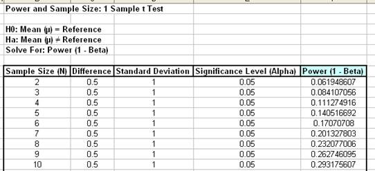
2. Ensure that Solve For Power (1 Beta) is selected. Select Sample Size (N) and Difference columns as shown. Enter the Standard Deviation value of 1. Enter .05 as the Significance Level value:


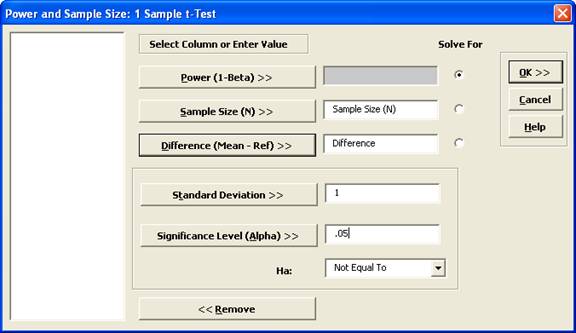
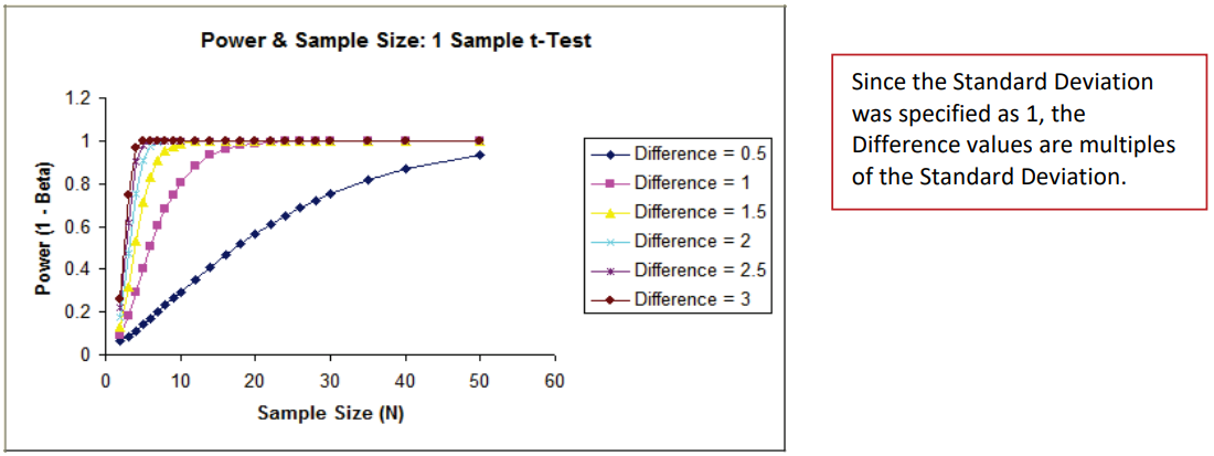
Note: By setting Standard Deviation to 1, the Difference values will be a multiple of Standard Deviation.

Click OK. The output report is shown below:



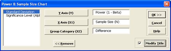
3. To create a graph showing the relationship between Power, Sample Size and Difference, click SigmaXL > Statistical Tools > Power & Sample Size Chart. Check Use Entire Data Table. Click Next.


4. Select Power (1 Beta), click Y Axis (Y); select Sample Size (N), click X Axis (X1); select Difference, click Group Category (X2). Click Add Title. Enter Power & Sample Size: 1 Sample t-Test:




5. Click OK. The resulting Power & Sample Size Chart is displayed: