How Do I Perform Multiple Regression in Excel Using SigmaXL?
Multiple Regression analyzes the relationship between one dependent variable (Y) and multiple
independent variables (X's). It is used to discover the relationship between the variables
and create an empirical equation of the form:
Y = b0 + b1*X1 + b2*X2 + ... + bn*Xn
This equation can be used to predict a Y value for a given set of input X values. SigmaXL
uses the method of least squares to solve for the model coefficients and constant term.
Statistical tests of hypothesis are provided for the model coefficients.
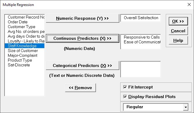
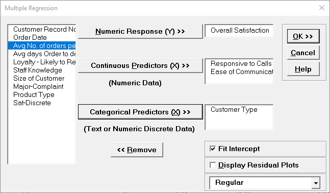
Open Customer Data.xlsx. Click Sheet 1
Tab. Click SigmaXL > Statistical Tools > Regression > Multiple
Regression. If necessary, click
Use Entire Data Table, click Next.
Select Overall Satisfaction, click Numeric
Response (Y) >>, select
Responsive to Calls and Ease of Communications, click
Continuous Predictors (X) >>.
Fit Intercept is checked by default. Check Display Residual
Plots as shown:
Note: Fit Intercept is optional. If unchecked the model will not
fit an intercept (constant) for the model. This is useful when you have strong a
priori reasons to believe that Y = 0 when the X or Xs are equal to 0 and the
relationship is linear. An example would be Y=automobile fuel consumption, X=automobile
weight.
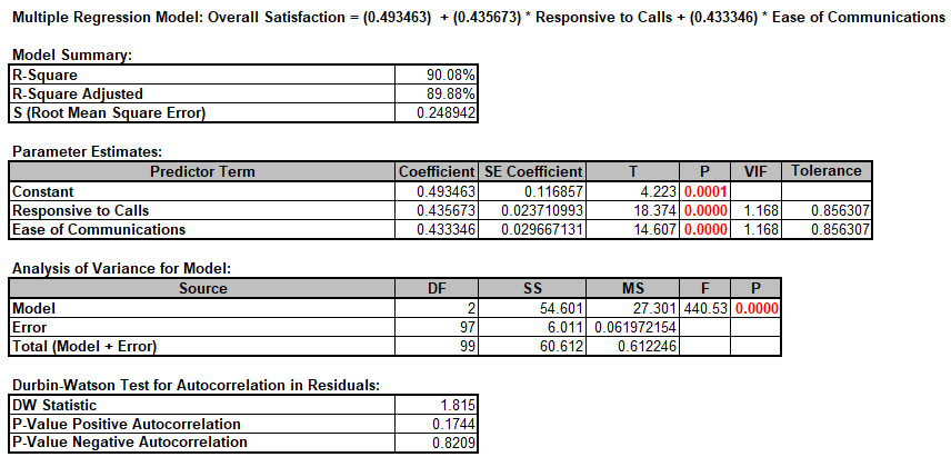
Click OK. The resulting
Multiple Regression report is shown:
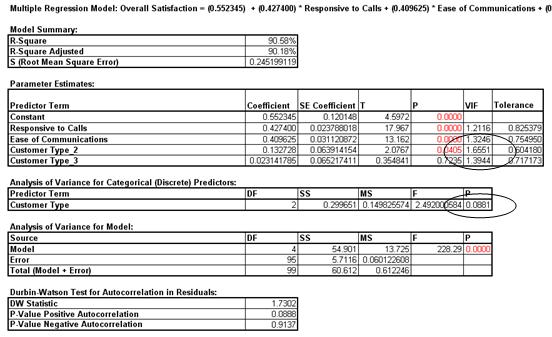
This model of Overall Satisfaction as a function of Responsiveness to Calls and Ease
of Communications looks very good with an R-Square value of 90%. Both Predictors are
shown to be significant with their respective p-values < .05. Clearly we need to
focus on these two X factors to improve customer satisfaction.
The variance inflation factor (VIF) and Tolerance scores are
used to measure multicollinearity or correlation among predictors. VIF = 1 indicates
no relation among predictors (which is highly desirable you will see examples of
this in Design of Experiments); VIF > 1 indicates that the predictors are
correlated; VIF > 5 indicates that the regression coefficients are strongly
correlated and this will lead to poor estimates of the coefficients. Tolerance =
1/VIF.
The Durbin-Watson Test is used to determine if the residuals
are autocorrelated. If either p-value is < .05, then there is significant
autocorrelation. This is likely due to an external bias factor affecting your
process over time (e.g. warm-up effect, seasonality). This will also be evident in
the plot of residuals versus observation order. Autocorrelation in the residuals is
not a problem for this model.
If the Fit Intercept option is unchecked, the following
diagnostics are not reported due to statistical issues associated with the removal
of the constant. These are: R-Square, R-Square Adjusted, VIF (Variance Inflation
Factor) and Tolerance collinearity diagnostics, DW (Durbin-Watson) autocorrelation
report, Anova report for Discrete factors (discrete factors will not be permitted
when "Fit Intercept" is unchecked). All other tests including residual diagnostics
are reported. Users can run the model with the "Fit Intercept" on to get the above
statistics and then run with "Fit Intercept" off.
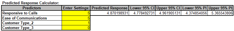
A predicted response calculator allows you to enter X values
and obtain the predicted response value, including the 95% confidence interval for
the long term mean and 95% prediction interval for individual values:
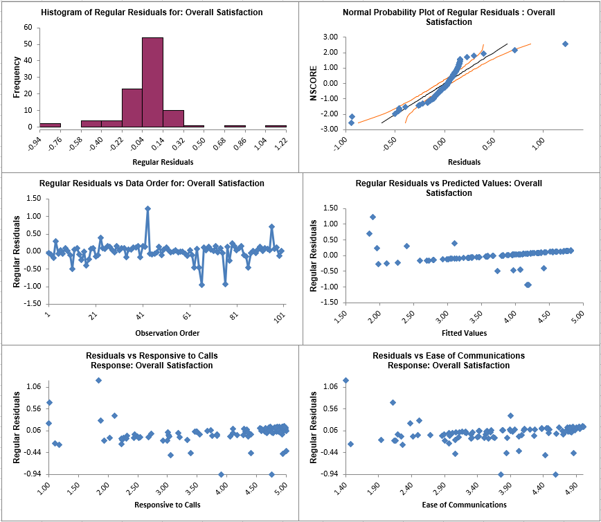
Click the Mult Reg Residuals Sheet and scroll right to view the
Residual Plots shown below:
Residuals are the unexplained variation from the regression model (Y - Ŷ). We
expect to see the residuals normally distributed with no obvious patterns in the
above graphs. Clearly this is not the case here, with the Residuals versus
Predicted Values indicating there is likely some other X factor influencing the
Overall Satisfaction. It would be appropriate to consider other factors in the
model.
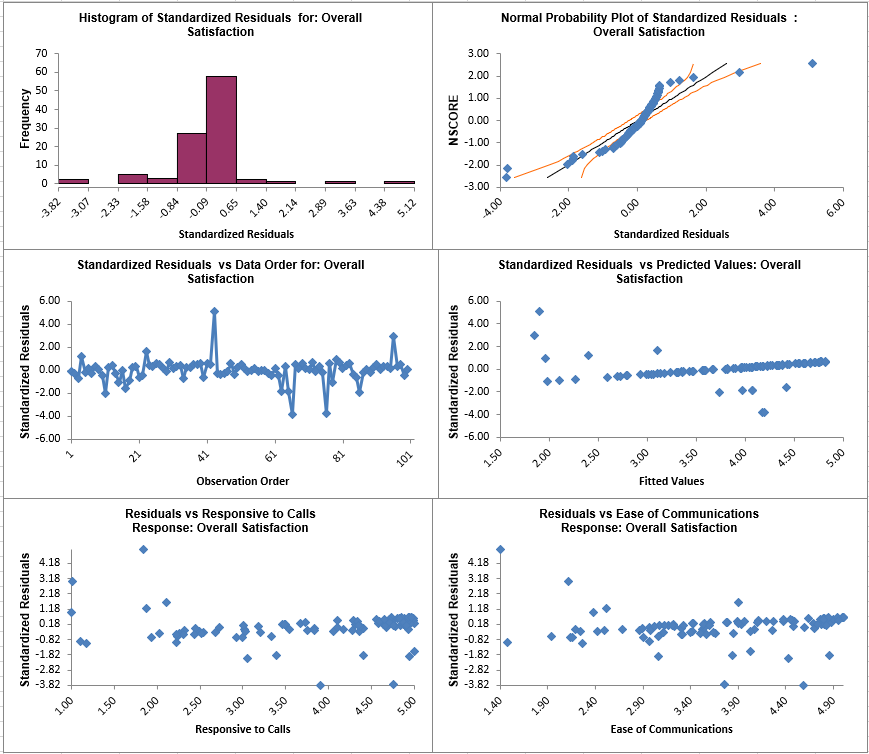
SigmaXL also provides Standardized Residuals and Studentized (Deleted t) Residuals. The
standardized residual is the residual, divided by an estimate of its standard deviation.
This makes it easier to detect outliers. Standardized residuals greater than 3 and less
than -3 are considered large (these outliers are highlighted in red). Studentized
deleted residuals are computed in the same way that standardized residuals are computed,
except that the ith observation is removed before performing the regression fit. This
prevents the ith observation from influencing the regression model, resulting in unusual
observations being more likely to stand out.
Click Recall Last Dialog (or press F3 ). Change the
Residual type to Standardized. Click OK. The resulting Standardized Residual plots are
displayed:
Other diagnostic measures reported but not plotted include Leverage, Cook's Distance
(Influence), and DFITS. Leverage is a measure of how far an individual X predictor value
deviates from its mean. High leverage points can potentially have a
strong effect on the estimate of regression coefficients. Leverage values fall between 0
and 1. Cook's distance and DFITS are overall measures of influence. An observation is
said to be influential if removing the observation substantially changes the estimate of
coefficients. Cooks distance can be thought of as the product of leverage and the
standardized residual; DFITS as the product of leverage and the studentized residual.
The easiest way to identify observations with high leverage and/or influence is to plot
the measures on a run chart.
Multiple Regression with Continuous and Categorical Predictors
Click Recall Last Dialog (or press F3). Select
Customer Type, click Categorical Predictor (X) >>. We
will not discuss residuals further so you may wish to uncheck
Display Residual Plots. Keep Overall Satisfaction as the
Numeric Response (Y) and Responsive to Calls and
Ease of Communications as the Continuous Predictors (X):
Click OK. The resulting Multiple Regression report is shown:
The parameter estimates table now includes Customer Type 2 and Customer Type 3, but where is Customer Type 1? Since Customer Type is a discrete predictor, SigmaXL applies dummy coding (i.e. Customer Type 1 corresponds to Coded Variable 1 = 0 and Coded Variable 2 = 0; Customer Type 2 has Coded Variable 1 = 1 and Coded Variable 2 = 0; and Customer Type 3 has Coded Variable 1 = 0 and Coded Variable 2=1). Hence Customer Type 1 becomes the hidden or reference value. Other statistical software packages may use a different coding scheme based on -1,0,+1 instead of 0,1. The advantage of a 0,1 coding scheme is the relative ease of interpretation when making predictions with the model.
In the Predicted Response Calculator enter the settings as shown:
Note that for Customer Type 1, you would enter Customer Type 2 = 0 and Customer Type 3 = 0; for Customer Type 2, as shown, you entered Customer Type 2 = 1 and Customer Type 3 = 0; for Customer Type 3 you would enter Customer Type 2 = 0 and Customer Type 3 = 1.
Note the addition of the Analysis of Variance for Categorical (Discrete) Predictors. The Customer Type p-value is .08, so we do not have strong evidence to keep this term in the model. However, many practitioners will use an alpha value of 0.1 as a criterion for removal. You are probably wondering why the p-value for Customer Type is not lower given the results we saw earlier using ANOVA. The change in p-value is due to the inclusion of Responsive to Calls and Ease of Communications in the model. We have higher scores for Ease of Communications and Responsive to Calls with Customer Type 2. Statistically, Customer Type is somewhat correlated to Responsive to Calls and Ease of Communications (VIF for Customer Type = 1.66 and 1.39).