How Do I Perform Logistic Regression in Excel Using SigmaXL?
Binary Logistic Regression
Binary Logistic Regression is used to analyze the relationship between one binary dependent
variable (Y) and multiple independent numeric and/or discrete variables (X's). It is used to
discover the relationship between the variables and create an empirical equation of the
form:
Ln(Py/(1-Py)) = b0 + b1*X1 + b2*X2 + ... + bn*Xn
This equation can be used to predict an event probability Y value for a given set of input X
values. SigmaXL uses the method of maximum likelihood to solve for the model coefficients
and constant term. Statistical tests of hypothesis and odds-ratios are provided for the
model coefficients. The odds-ratios identify change in likelihood of the event for one unit
change in X.
An example application from medical research would be Y=Disease (Yes/No) and Xs = Age,
Smoker (Yes/No), Number Years of Smoking and Weight. The model coefficient p-values would
indicate which Xs are significant and the odds-ratios would provide the relative change in
risk for each unit change in X.
We will analyze the familiar Customer Satisfaction data using Y=Discrete Satisfaction where
the values have been coded such that an Overall Satisfaction score >= 3.5 is considered a 1,
and scores < 3.5 are considered a 0. Please note, we are not advising that continuous data
be converted to discrete data in actual practice, but simply using the Discrete
Satisfaction score for continuity with the previous analysis.
Open Customer Data.xlsx. Click Sheet 1 Tab (or
press
F4 to activate last worksheet). Click SigmaXL >
Statistical Tools > Regression > Binary Logistic Regression.
If necessary, click Use Entire Data Table, click
Next.
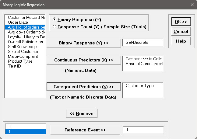
Select Sat-Discrete, click Binary Response (Y)
>>; select Responsive to Calls and Ease of
Communications, click Continuous Predictors (X)
>>; select Customer Type, click Categorical
Predictors (X) >>.
Note that Response Count (Y)/Sample Size (Trials) should be
used when each record contains both the number of occurrences along with
associated sample size.
This is common when tracking daily quality data or performing design of
experiments where each run contains a response of the number of defects and
sample size.
Click OK.
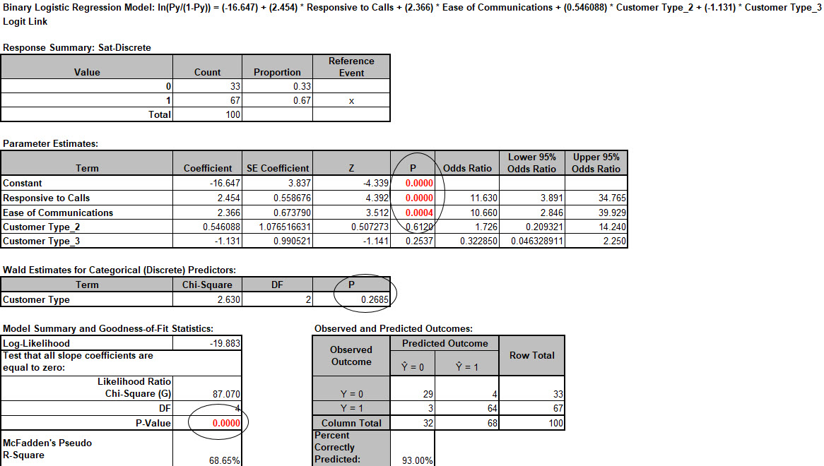
The resulting Binary Logistic Regression report is shown:
The Likelihood Ratio p-value < .05 tells us that the model is significant.
The p-values for the coefficients in the Parameter Estimates table confirm that
Responsive to Calls and Ease of Communications are significant.
The p-value in Wald Estimates for Categorical (Discrete) Predictors table tells
us that Customer Type is not significant here.
Tip: Significance for categorical predictors should be based on
the Wald Estimates not the p-values given in the Parameter Estimates table.
Note that Customer Type 1 is not displayed in the Parameter Estimates table.
This is the "hidden" reference value for Customer Type.
Categorical predictors must have one level selected as a reference value.
SigmaXL sorts the levels alphanumerically and selects the first level as the
reference value.
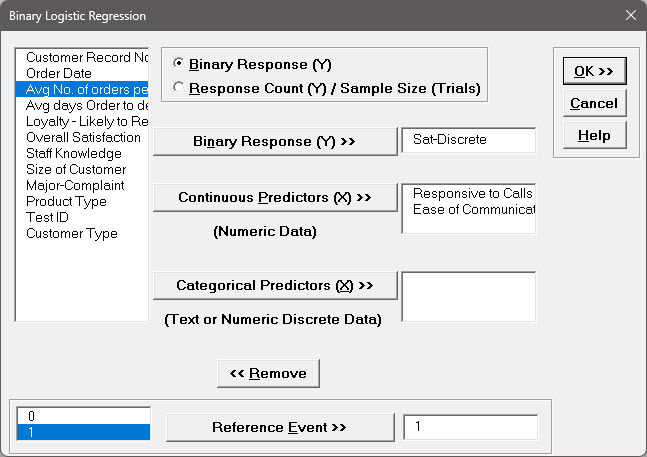
Now we will rerun the binary logistic regression but remove Customer
Type as a predictor.
Press F3 or click Recall SigmaXL Dialog to
Recall Last Dialog.
Remove Customer Type by highlighting Customer Type and
double-clicking (or press the Remove button).
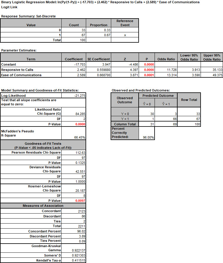
Click OK. The resulting Binary Logistic report is shown:
The Odds Ratios in the Parameter Estimates table tell us that for every unit
increase in Responsive to Calls we are 11.7 times more likely to obtain a
satisfied customer.
For every unit increase in Ease of Communications we are 13.3 times more likely
to obtain a satisfied customer.
McFaddens Pseudo R-Square mimics the R-square found in linear regression.
This value varies between 0 and 1 but is typically much lower than the
traditional R-squared value.
A value less than 0.2 indicates a weak relationship; 0.2 to 0.4 indicates a
moderate relationship; greater than 0.4 indicates a strong relationship.
Here we have an R-square value of 0.66 indicating a strong relationship.
This is also confirmed with the Percent Correctly Predicted value of 96%.
The Pearson, Deviance and Hosmer-Lemeshow Goodness of Fit tests are used to
confirm if the binary logistic model fits the data well. P-values < .05 for
any of these tests indicate a significant lack of fit. Here the Hosmer-Lemeshow
test is indicating lack of fit. Residuals analysis will help us to see where the
model does not fit the data well.
The measures of association are used to indicate the relationship between the
observed responses and the predicted probabilities. Larger values for
Goodman-Kruskal Gamma, Somers D and Kendalls Tau-a indicate that the model has
better predictive ability.
The residuals report is given on the Sheet Binary Logistic
Residuals.
Three types of residuals are provided: Pearson, Standardized Pearson and
Deviance.
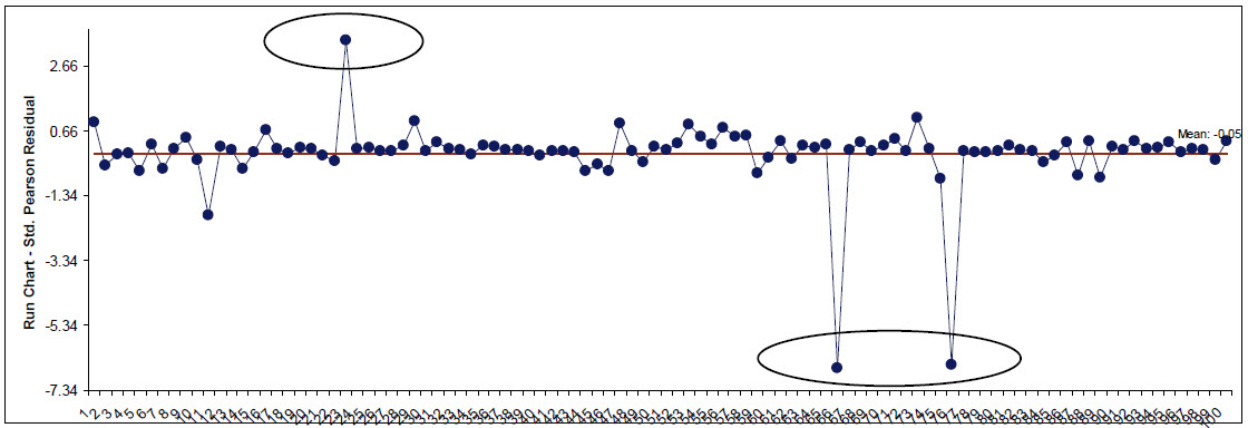
The Standardized Pearson Residual is most commonly used and is shown here
plotted on a Run Chart.
To create, click SigmaXL > Graphical Tools > Run Chart,
check Use Entire Data Table to select the Residuals
data, click Next, select Std. Pearson Residual as the
Numeric Data Variable (Y). Click OK.
Any Standardized Pearson Residual value that is less than -3 or greater than +3
is considered extreme and should be investigated.
There are 3 such outliers here: rows 24, 67, and 77 in the residuals table.
The +3.4 value indicates that the predicted event probability was low (.08) but
the actual result was a 1.
The -6.6 value indicates that the predicted event probability was high (.98) but
the actual result was a 0.
The large negative residuals have high Responsive to Calls and Ease of
Communications but dissatisfied customers.
The reasons for these discrepancies should be explored further but we will not
do so here.
Reselect the Binary Logistic Report sheet.
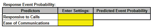
Scroll over to display the Event Probability calculator:
This calculator provides a predicted Event Probability for given values of X (in
this case the probability of a satisfied customer). Enter the values 3,3; 4,4;
5,5 as shown:
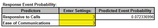
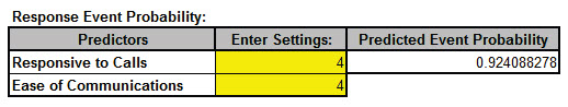
If Responsive to Calls and Ease of Communications are both equal to 3, the
probability of a satisfied customer is only .07 (7%); if Responsive to Calls and
Ease of Communications are both equal to 5, the probability of a satisfied
customer is .9995 (99.95%)
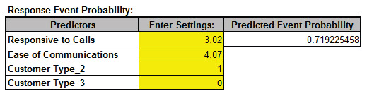
Note that if the calculator includes predictors that are categorical (discrete),
enter a 0 or 1 to denote the selected level as shown below (using the original
analysis which included Customer Type):
If we wanted to select Customer Type 1, enter a 0 for both Customer
Types 2 and 3.
Customer Type 1 is the hidden reference value.
Ordinal Logistic Regression
Ordinal Logistic Regression is used to analyze the relationship between one ordinal
dependent variable (Y) and multiple independent continuous and/or discrete variables
(X's).
We will analyze the Customer Satisfaction data using Y=Loyalty Likely to Recommend
score which contains ordinal integer values from 1 to 5, where 5 indicates that the
customer is very likely to recommend us and 1 indicates that they are very likely to
not recommend us.
Open Customer Data.xlsx.
Click Sheet 1 Tab (or press F4 to activate
last worksheet).
Click SigmaXL > Statistical Tools > Regression > Ordinal
Logistic Regression.
If necessary, click Use Entire Data Table, click
Next.
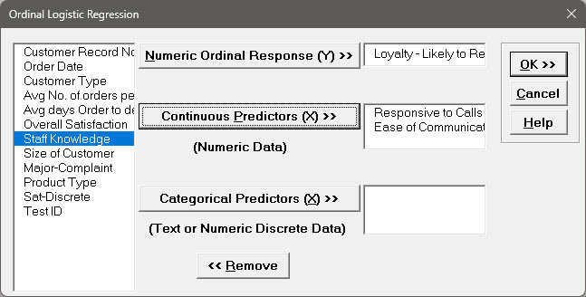
Select Loyalty Likely to Recommend, click Numeric Ordinal
Response (Y) >>; select Responsive to Calls and
Ease of Communications, click Continuous Predictors (X)
>>.
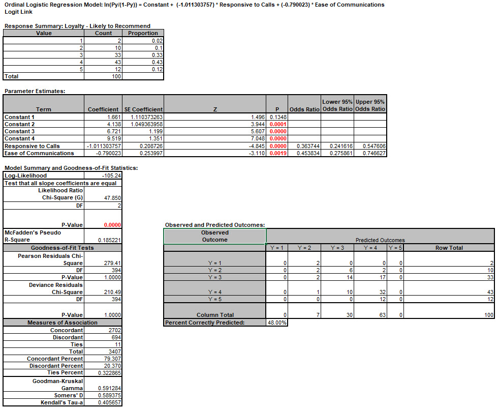
Click OK. The resulting Ordinal Logistic report is shown:
The Likelihood Ratio p-value < .05 tells us that the model is significant.
The low p-values for the coefficients confirm that Responsive to Calls and Ease
of Communications are significant.
The Odds Ratios tell us that for every one-unit increase in Responsive to Calls
the chance of a Loyalty score of 1 versus 2 (or 2 versus 3, etc.) is reduced by
a multiple of 0.36.
This is not very intuitive but will be easy to see when we use the Response
Outcome Probability calculator.
McFaddens Pseudo R-Square value is 0.185 indicating that this is a weak (but
close to moderate) degree of association. This is also confirmed with the
Percent Correctly Predicted value of 48%.
The Pearson and Deviance Goodness of Fit (GOF) tests are used to confirm if the
ordinal logistic model fits the data well.
P-values < .05 would indicate a significant lack of fit.
Given that the GOF p-values are greater than .05, we conclude that there is no
significant lack of fit.
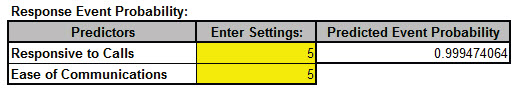
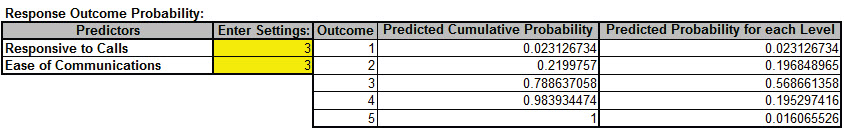
Scroll across to the Response Outcome Probability calculator.
This calculator provides predicted outcome (event) probabilities for given
values of X (in this case the probability of a satisfied customer).
Enter the values 3,3; 4,4; 5,5 as shown:
Referring to the Predicted Probability for each Level, if
Responsive to Calls and Ease of Communications
are both equal to 3, we would expect to see typical loyalty scores of 3 (57%)
with some at 2 (20%) and 4 (20%);
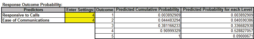
if Responsive to Calls and Ease of
Communications are both equal to 4, we would expect typical loyalty
scores of 4 (53 %) with some at 3 (34%) and 5 (9%);
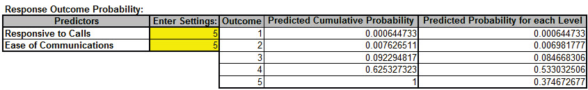
if Responsive to Calls and Ease of
Communications are both equal to 5, we would expect typical loyalty
scores of 4 (53 %) with some at 3 (8.5%) and 5 (37.5%).