Example 11: Multiple Response Optimization – Tire Tread Compound
Derringer and Suich [3] demonstrate the use of the Desirability function with the famous Tire Tread Compound example. The controllable factors are:
X1: Hydrated silica level: Silica is a fine powder added to rubber to improve strength and reduce rolling resistance (which affects fuel efficiency). Hydrated silica has water molecules bound to it, influencing how it mixes and bonds with the rubber.
X2: Silane coupling agent level: Silane is a chemical that acts like a "glue" to bond silica particles to the rubber molecules, enhancing overall compound integrity and performance under stress.
X3: Sulfur level: Sulfur is a key vulcanizing agent in rubber production—it creates cross-links between polymer chains during heating (vulcanization), making the rubber more elastic and durable.
The level settings are given as coded -1/+1. The experiment is a 20 Run Central Composite with alpha = 1.633.
The four responses, goals and upper/lower limits are:
Y1: PICO abrasion index: A measure of wear resistance - higher values mean the tread lasts longer against road friction. The goal is to Maximize Y1. The Lower Limit is a specification limit = 120, with any Y1 value < 120 resulting in an unacceptable tire tread compound. The Upper Limit is 170, which is set from a practical standpoint, we consider any PICO Abrasion Index above 170 to be only as desirable as one at 170.
Y2: 200% modulus: Indicates the stiffness of the rubber when stretched to twice its original length. Higher values suggest better strength and load-bearing capacity, important for handling and stability. The goal is to Maximize Y2. The Lower Limit is a specification limit = 1000 and the practical upper limit is 1300.
Y3: Elongation at break: The percentage stretch the material can endure before snapping. The goal is to hit a Target = 500 with Lower Limit = 400 and Upper Limit = 600, balancing flexibility (to absorb shocks) with toughness (to avoid premature failure).
Y4: Hardness: A scale measuring surface resistance to indentation. The goal is to hit a Target = 67.5 with Lower Limit = 60 and Upper Limit = 75. Too soft, and the tire wears quickly; too hard, and it loses grip on wet roads.
In SigmaXL Importance allows for weighting of the responses according to their relative importance. The default setting of 1 matches what was used in the paper. Weight is a shape factor. For weight = 1, the desirability function increases linearly. This default setting matches what was used in the paper.
We will also demonstrate new features in SigmaXL Version 11.1: Historical DOE, Evaluate Historical DOE, Overlaid Contour Plots, Desirability Contour Plots and the MRO Calculator.
-
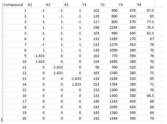
Open the file Tires DOE Derringer Suich.xlsx. This is the data from Table 1 Experimental Design.
-
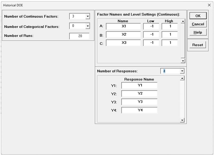
We will convert this data into a Historical DOE. Click SigmaXL > Design of Experiments > Advanced Design of Experiments: Historical Design of Experiments > Historical DOE. Select Number of Continuous Factors = 3, Number of Categorical Factors = 0, Number of Runs = 20. Enter Factor Names as X1, X2, X3. Specify Number of Responses = 4 as shown.
-
Click OK.
-
Select cells B2:H21 in Sheet 1 of Tires DOE Derringer Suich.xlsx.
-
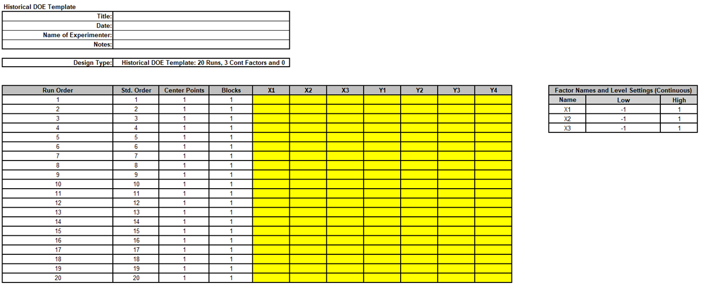
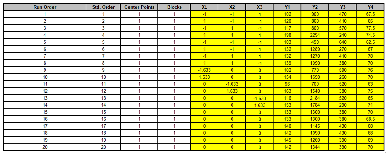
Copy/Paste Values into the yellow highlighted region of the Historical DOE Template.
-
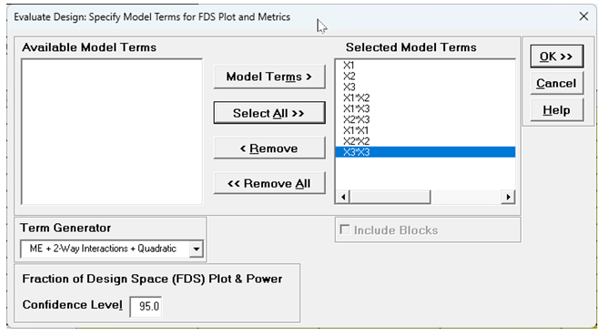
When using Historical DOE, it is recommended that the design be evaluated before proceeding with analysis. Click SigmaXL > Design of Experiments > Advanced Design of Experiments: Evaluate Design.
-
Select Model Terms as shown
-
Click OK.
-
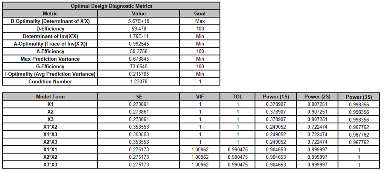
The VIF scores look good all at 1 or close to 1, showing no multicollinearity. The G-Efficiency = 73.7% is excellent, and the condition number is low. This is what would be expected since the design was a central composite.
-
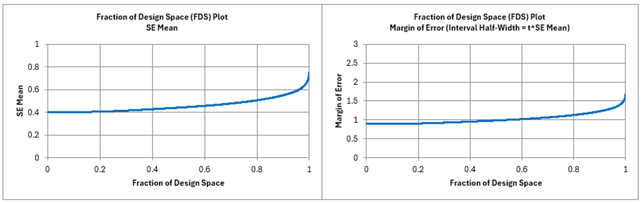
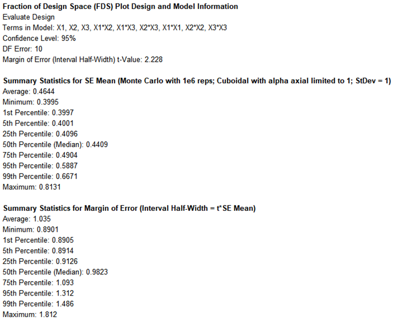
Power(2S) which is the power to detect an effect size = 2*StDev, looks good for the main effects and quadratic terms, but the interaction terms are lower than we would like (< 0.8). However, power for a Response Surface Design is not as important as the prediction error given by the FDS Plot, which is acceptable given that this is a Uniform Precision Central Composite Design with a benchmark 95th Percentile Margin of Error value = 1.31.
-
Now we are ready to Analyze. Click on the Sheet Historical DOE. Click SigmaXL > Design of Experiments > Advanced Design of Experiments: Historical Design of Experiments > Analyze Historical DOE.
-
Select Responses and Model Terms as shown with Term Generator as ME + 2-Way Interactions + Quadratic. Uncheck Residual Plots:
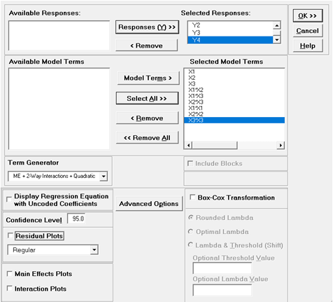
-
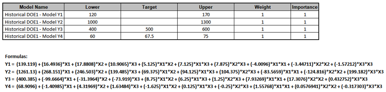
Click OK. The Multiple Regression reports are given for Y1 to Y4.
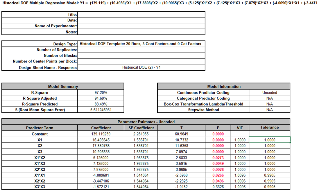
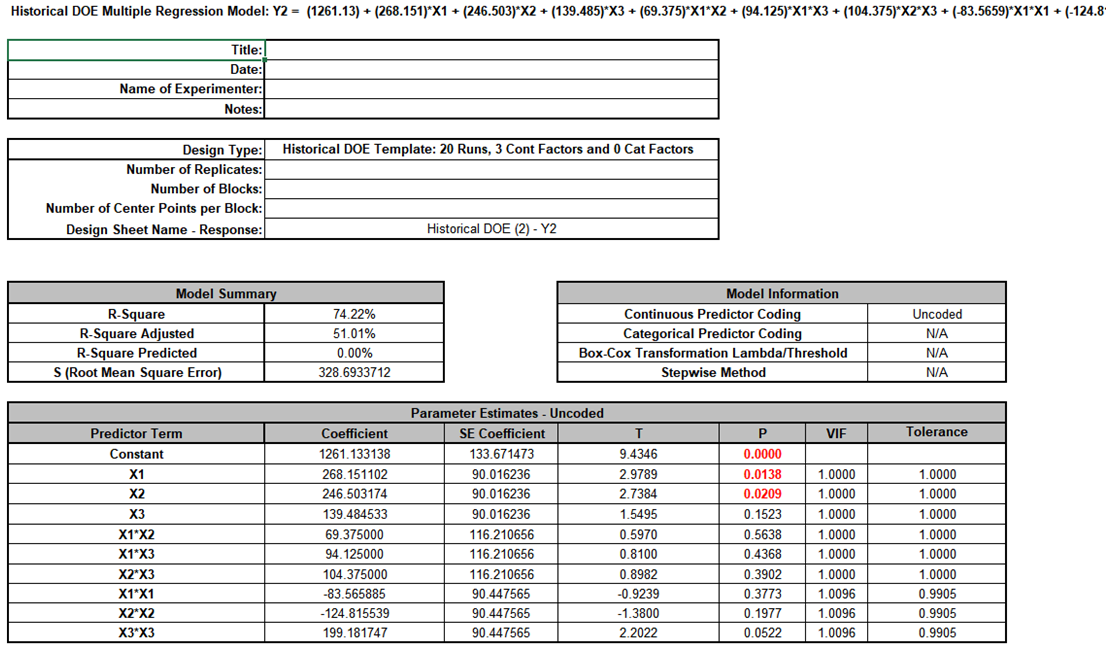
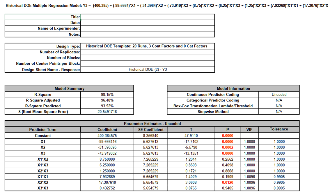
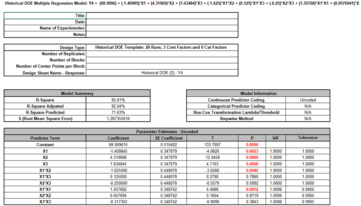
The Coefficients and model S (RMSE) all agree with those given in Table 2 of the paper.
-
We will not do any model refinement as that was not done in the paper.
-
Now we are ready to run Multiple Response Optimization. Click SigmaXL > Design of Experiments > Advanced Design of Experiments: Historical Design of Experiments > Multiple Response Optimization.
-
Select Responses as shown. Set Goal, Lower, Target and Upper as shown. Check Overlaid Contour Plots and Desirability Contour Plots.
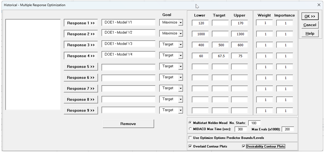
In the previous example we selected MIDACO. In this example Multistart Nelder-Mead is used as it gives the same solution result as given in the paper and MIDACO does not improve on it. For more information on the MRO options, see Multiple Response Optimization Dialog.
-
Click OK. This will take about 1 minute:
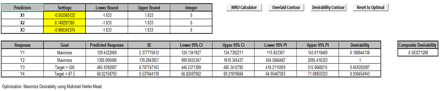
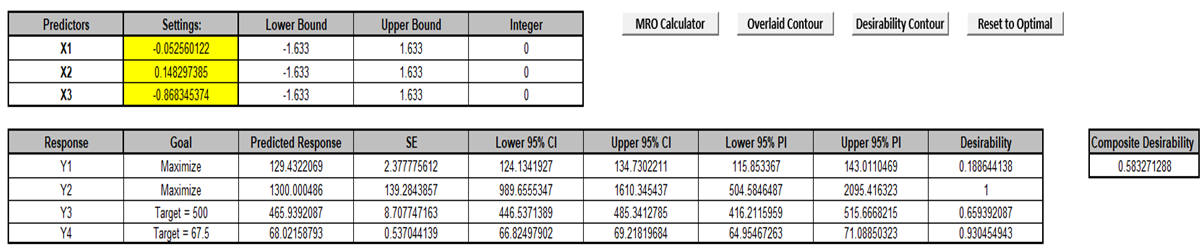
The maximum composite desirability = 0.583 matches the value obtained in the paper (Table 3).
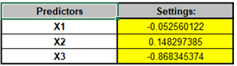
The coded optimal settings to obtain this are: X1 (Hydrated silica level) = -.053; X2 (Silane coupling agent level) = 0.148 and X3 (Sulfur level) = -0.868, very close to the values obtained in the paper.
The predicted response for Y1 (PICO abrasion index) = 129.4 (with 95% CI: 124.1 to 134.7). The desirability for Y1 (d1) = 0.189.
The predicted response for Y2 (200% modulus) = 1300.0 (with 95% CI: 989.7 to 1610.3). The desirability for Y2 (d2) = 1.
The predicted response for Y3 (Elongation at break) = 465.9 (with 95% CI: 446.5 to 485.3). The desirability for Y3 (d3) = 0.66.
The predicted response for Y4 (Hardness)= 68.02 (with 95% CI: 66.82 to 69.22). The desirability for Y4 (d4) = 0.93.
The input settings can be changed (in the yellow highlight region). If the values are changed, the Predicted Response values, Desirability values and Composite Desirability will be cleared. Click the MRO Calculator button to recalculate the new values.
-
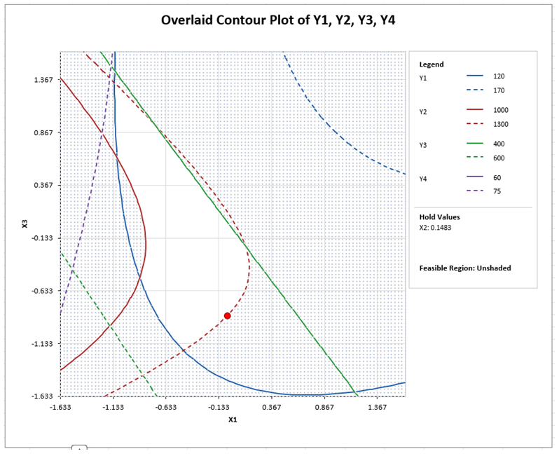
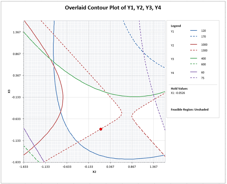
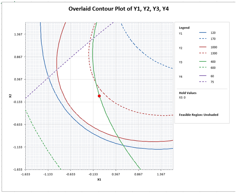
Click on the Sheet Overlaid Contour Plots. An Overlaid Contour Plot is created for every pairwise combination of continuous factors and other factors held fixed at their optimal values. The contour lines are the response upper and lower bounds, with the feasible region that satisfies all bounds unshaded and the optimal point shown as a red dot. This is a powerful graphical complement to the multiple response optimization.
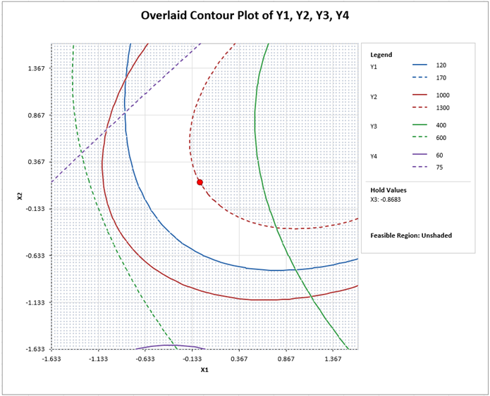
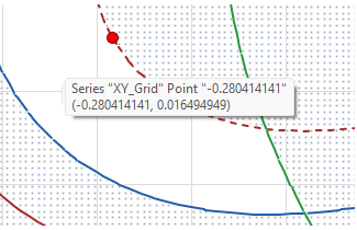
If you hover the mouse cursor on the red dot you will see the XY values for the optimum value computed by MRO.
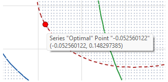
You can also hover the mouse cursor anywhere on the plot to obtain XY values. This uses a transparent 100x100 grid.
Using the mouse cursor to explore the feasible (or infeasible) region, other input combinations may be considered and entered into the MRO Calculator.
-
For example, click the MRO Calculator Sheet, enter the center point values in the yellow highlight region as shown and press the MRO Calculator button for the updated predicted response values and desirability values.
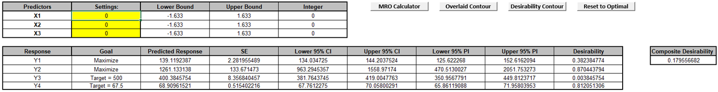
This is a degradation of the Composite Desirability.
-
Press the Overlaid Contour button to recreate the Overlaid Contour Plots with these center point settings.
-
Having explored the center points and determined that they are sub-optimal, we will now restore the optimal settings by clicking the Reset to Optimal button.
-
Click on the Sheet Desirability Plots. A Desirability Contour/Surface Plot is created for every pairwise combination of continuous factors and other factors held fixed at the optimal values (all hold values are given). The contour lines are composite desirability values. This is used to assess solution robustness, ideally looking for a flat response close to the optimal value.
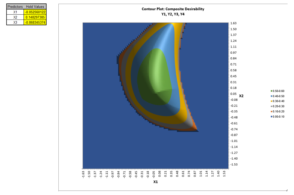
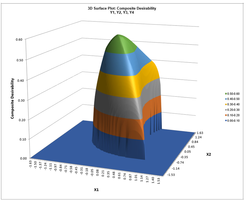
Looking at the X1-X2 Contour and Surface Plots, we see the region where all desirability values are greater than 0.5, giving a robust region where the X1 and X2 values can deviate slightly while maintaining a composite desirability greater than 0.5. This agrees with the composite desirability contour plot given in the paper. The X1-X3 and X2-X3 Contour and Surface Plots can also be reviewed, but we will not do so here.
Tip: Excel does not permit mouse hover on the contour or surface plots, but the following demonstrates how you can view the data to get a detailed view of the desirability values. Click on the contour plot, right mouse click, Select Data:
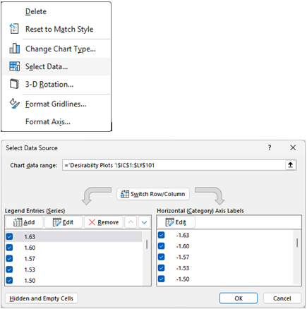
Click Cancel. Select Cell ID2, which is the upper left desirability value used in the Contour Plot.
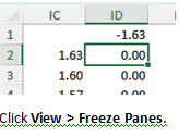
Now scroll over to view the Optimal values as given in the MRO Calculator:
Note that the columns are used for the chart X Axis, which is X1 here. The rows are used for the chart Y Axis, which is X2 here. The nearest X1 Column is JZ, which is -0.05 (top frozen row). The nearest X2 Row is 47 which is 0.15 (first frozen column). Click on cell JZ47 and reduce the zoom to 80%.
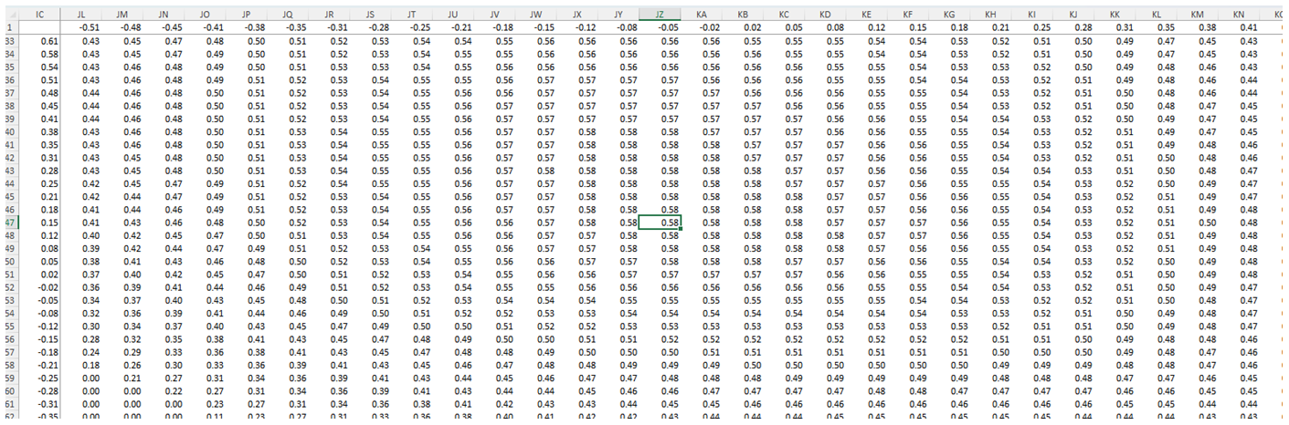
This gives a detailed view of the X1, X2 and Z desirability values around the optimal point.
Note that Column LZ is the start of the X2 X3 Contour Plot.
Conditional formatting may also be applied, but we will not do so here.
When done, be sure to unfreeze the panes: View > Freeze Panes > Unfreeze Panes. Scroll all the way left and up to view the Contour Plot. Restore the zoom to 100%.


