How Do I Perform Equal Variance Tests (Bartlett, Levene and Welch's
ANOVA) in Excel Using SigmaXL?
Bartlett's Test
Bartlett's Test is similar to the 2 sample F-Test (SigmaXL > Statistical Tools > 2 Sample
Comparison Test) but allows for multiple group comparison of variances (or standard
deviations). Like the F-Test, Bartlett's requires that the data from each group be normally
distributed but is more powerful than Levene's Test.
Open Delivery Times.xlsx, click on Sheet 1 tab.
Click SigmaXL > Statistical Tools > Equal Variance Tests >
Bartlett. Ensure that the entire data table is selected. If not, check
Use Entire Data Table.
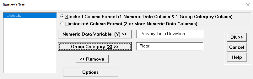
Click Next. Ensure that Stacked Column Format is
checked. Select
Delivery Time Deviation, click Numeric Data Variable (Y)
>>; select
Floor, click Group Category (X) >>.
Click OK. The results are
shown below:
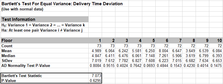
All 10 Anderson-Darling Test P-Values are > .05 indicating that
all group data are normal. Since
the assumption of normality is met, Bartlett's is the appropriate test to use. If any
one of the
groups have a low P-Value for the Normality test, then Levene's test should be used.
With the p-value = 0.63 we fail to reject H0; we do not have
evidence to show that the group variances are unequal (practically speaking we will
assume that the variances are equal).
If the Equal Variance test is only being used to test the
assumption for use in ANOVA then it is
not necessary to examine the Multiple Comparison of Variances. However, in the context
of a process improvement project, we often do want to know which groups are
significantly different. This can give us important clues to identify opportunities for
variance reduction.
With a Fail-to-Reject H0 it is unnecessary to review the Multiple
Comparison of Variances or the ANOM Variances Chart, but we will do so here for
demonstration purposes.
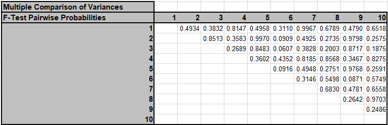
The default Multiple Comparison of Variances is a matrix of F-Test
Pairwise Probabilities:
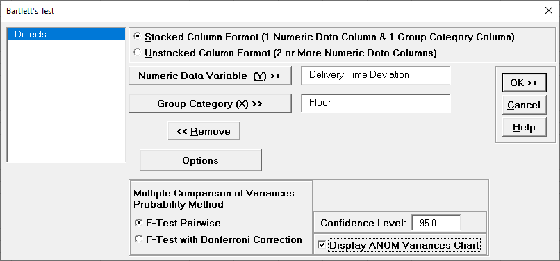
Press F3 or click
Recall SigmaXL Dialog to Recall Last Dialog. Click
Options. Check Display ANOM Variances Chart.
Note: The Confidence Level
determines the alpha level (alpha = (100 CI)/100) used to highlight the P-Values
and the alpha level for the ANOM chart. However, the alpha level used to highlight
P-Values in the Anderson-Darling Normality Test is always 0.05.
We will not run F-Test with Bonferroni Correction
in this example, but typically that would be used when there are more than 3
groups.
Click OK. Click
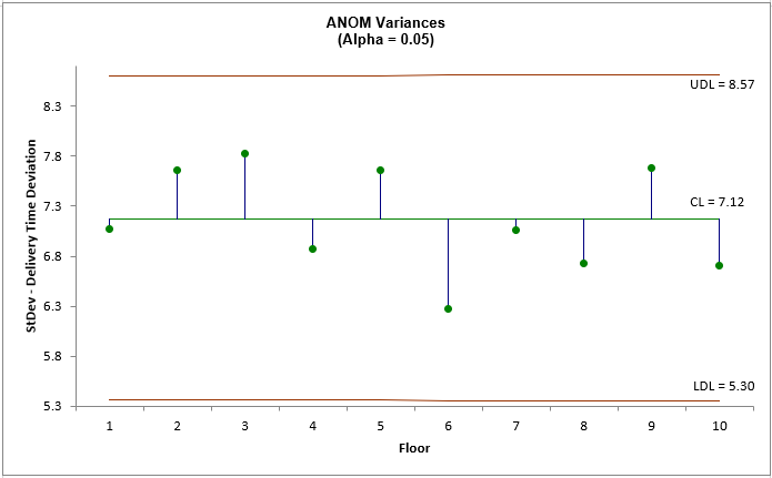
ANOM_Variances sheet tab to display the ANOM Chart:
The ANOM Variances chart visually shows that none of the
group standard deviations are significantly different from the grand mean of all the
standard deviations. It is called an ANOM
Variances Chart but displays Standard Deviations for ease of interpretation (similar
to a Standard Deviation S Control Chart). This does, however, result in
non-symmetrical decision limits. The ANOM Variances chart in
SigmaXL > Graphical Tools > Analysis of Means (ANOM) >
ANOM Variances has an option to display Variances.
Levene's Test
Levene's Test for multiple group comparison of variances is less powerful that Bartlett's
Test, but is robust to the assumption of normality. (This is a modification of the original
Levene's Test, sometimes referred to as the Browne-Forsythe Test).
Open Customer Data.xlsx, click on Sheet 1 tab.
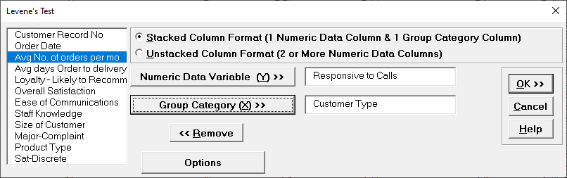
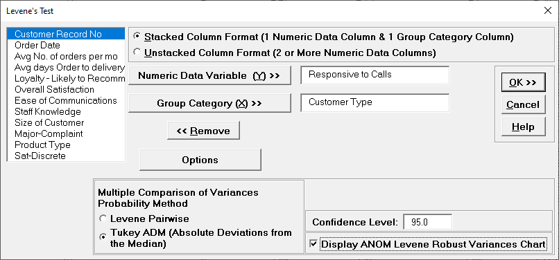
Click SigmaXL > Statistical Tools > Equal Variance Tests >
Levene. Ensure that the entire data table is selected. If not, check
Use Entire Data Table.
Click
Next. Ensure that Stacked Column Format is checked.
Select
Responsive to Calls, click Numeric Data Variable (Y) >>;
select
Customer Type, click Group Category (X) >>.
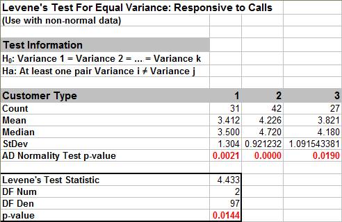
Click OK. The results
are shown below:
The Levene's Test p-value of 0.0144 tells us that we reject H0. At least one pairwise
set of variances are not equal. The normality test p-values indicate that all 3 groups
have non-normal data (p-values < .05). Since Levene's Test is robust to the
assumption of normality, it is the correct test for equal variances (rather than
Bartlett's Test).
Now that we have determined that the variances (and standard deviations) are not equal,
we are presented with a problem if we want to apply classical One-Way ANOVA to test for
equal group means. ANOVA assumes that the group variances are equal. A modified ANOVA
called Welch's ANOVA can be used as an alternative here.
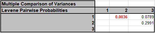
The default Multiple Comparison of Variances is a matrix of Levene Pairwise
Probabilities:
Customer Type 1 versus Customer Type 2 shows a significant
difference in variance. Press F3 or click Recall SigmaXL
Dialog to Recall Last Dialog. Click Options. Select
Tukey ADM (Absolute Deviations from Median). Check Display ANOM
Levene Robust Variances Chart.
Note: The Confidence Level
determines the alpha level (alpha = (100 CI)/100) used to highlight the P-Values and
the alpha level for the ANOM chart. However, the alpha level used
to highlight P-Values in the Anderson-Darling Normality Test is always
0.05.
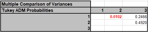
Click OK. The Multiple Comparison of Variances is a matrix of Tukey ADM
Probabilities:
The 1 2 P-Value is significant but larger than the Levene
Pairwise because it adjusts for the family-wise error rate. Note that it is smaller than
the Bonferroni corrected value = .0036 * 3 = .011, so more powerful than Bonferroni. The
difference in power between Tukey and
Bonferroni becomes more prominent with a larger number of groups, so Bonferroni is not
included as an option.
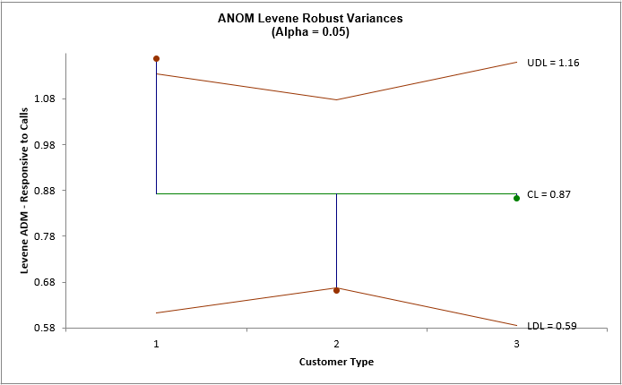
Click the ANOM_Levene sheet tab to display the ANOM Chart:
The ANOM chart clearly shows Customer Type 1 has significantly higher variance (ADM)
than overall and Customer Type 2 has significantly lower variance.
The varying decision limits are due to the varying sample sizes for each Customer Type,
with smaller sample size giving wider limits in a manner similar to a control chart. If
the data are
balanced, the decision limit lines will be constant.
Now that we have determined that the variances are not equal, we are presented with a
problem if we want to test for equal group means. Classical ANOVA assumes that the group
variances are equal, so should not be used. A modified ANOVA called Welch's ANOVA is
robust to the assumption of equal variances and will be demonstrated next.
Welch's Anova Test
Welch's ANOVA is a test for multiple comparison of means. It is a modified One-Way ANOVA that
is robust to the assumption of equal variances. Welch's ANOVA is an extension of the 2
sample t-test for means, assuming unequal variance. Nonparametric methods could also be used
here but they are not as powerful as Welch's ANOVA.
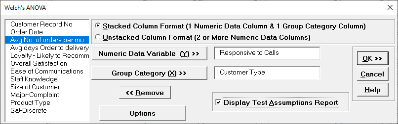
Open Customer Data.xlsx, click on Sheet
1 tab.
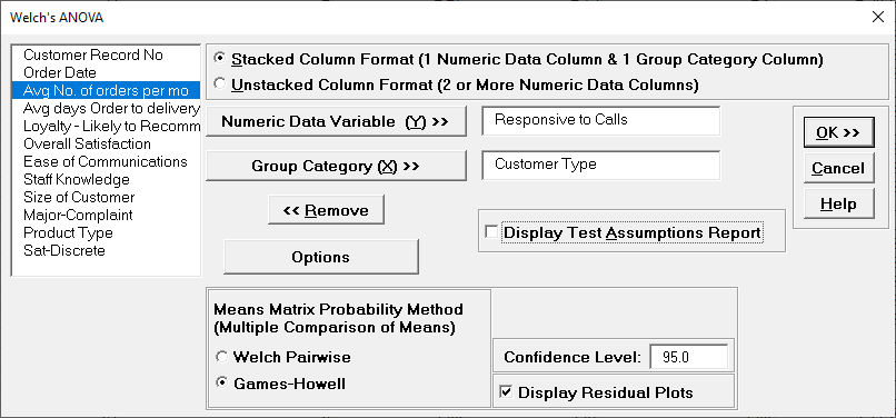
Click SigmaXL > Statistical Tools > Equal Variance
Tests > Welch's ANOVA. Ensure that the entire data table is selected. If
not, check
Use Entire Data Table.
Click Next. Ensure that Stacked Column
Format is checked. Select Responsive to Calls, click
Numeric Data Variable (Y) >>; select Customer Type,
click
Group Category (X) >>.
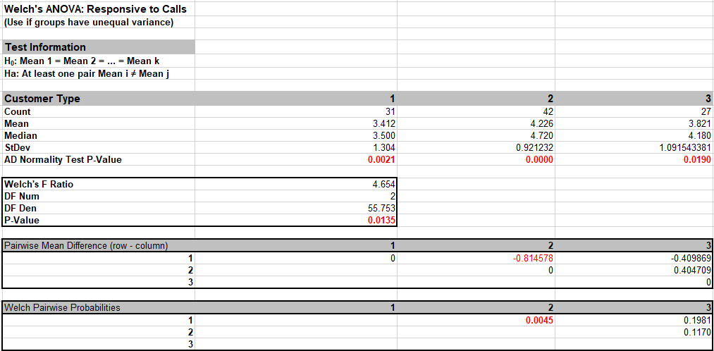
Click OK. The results are shown below:
The p-value for Welch's ANOVA is 0.0135, therefore we reject H0 and
conclude that the group means for Responsive to Calls are not equal. We will explore the
relationship between Overall Satisfaction and Responsive to Calls later.
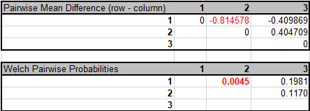
From the Pairwise Mean Difference (Means Matrix), we conclude that
Mean Responsive to Calls is significantly different between Customer Type 1 and 2. Note
that the default probabilities are Welch Pairwise. See below for more details on the
multiple comparison options.
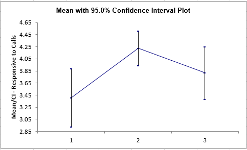
A graphical view of the Responsive to Calls Mean and 95% Confidence
Intervals are given to complement the Means Matrix. Note that the standard deviations
are unpooled, resulting in different CI widths for each group. The fact that the CIs
for Customer Type 1 do not overlap
those of Type 2, visually shows that there is a significant difference in mean
Responsive to Calls. The overlap of CIs for Type 2 and 3 shows that the mean scores for
2 and 3 are not significantly different.
Later, we will explore the relationship between Responsive to Calls
and Overall Satisfaction.
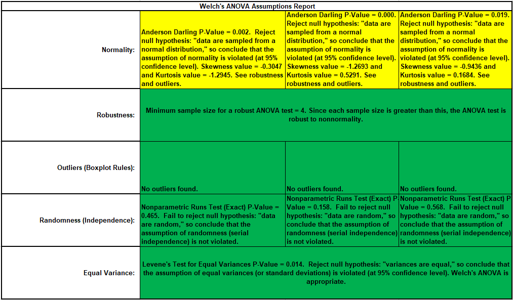
Welch's ANOVA Assumptions Report:
This is a text report with color highlight: Green (OK), Yellow
(Warning) and Red (Serious Violation).
Each sample is tested for Normality using
the Anderson-Darling test. If not normal, the minimum sample size for robustness of the
ANOVA Test is determined utilizing Monte Carlo
regression equations (see Basic Statistical Templates — Minimum Sample Size for Robust
t-Tests and ANOVA). If the sample size is inadequate, a warning is given and the
appropriate Nonparametric test is recommended (Kruskal-Wallis if there are no extreme
outliers, Mood's Median if there are extreme outliers).
Each sample is tested for Outliers defined as: Potential: Tukey's Boxplot (> Q3 +
1.5*IQR or < Q1 − 1.5*IQR); Likely: Tukey's Boxplot 2.2*IQR; Extreme: Tukey's Boxplot
3*IQR. If outliers are present, a warning is given and recommendation to review the data
with a Boxplot and Normal Probability Plot.
Tip: If the removal of outlier(s) result in an Anderson-Darling P-Value
that is > 0.1, a notice is given that excluding the outlier(s), the sample data are
inherently normal.
Each sample is tested for Randomness using the Exact
Nonparametric Runs Test. If the sample data is not random, a warning is given and
recommendation to review the data with a Run Chart.
A test for Equal Variances is also applied. If all sample data are normal, Bartlett's
Test is utilized, otherwise Levene's Test is used. Since we are using Welch's ANOVA, it
is confirmed as appropriate.
Press F3 or click Recall SigmaXL
Dialog to Recall Last Dialog. Uncheck Display Test Assumptions
Report. Click the Options button. Select
Games-Howell. Check
Display Residual Charts as shown:
Note: The Confidence Level is
used to set the level in the Mean/Confidence Interval Plot and the alpha level (alpha =
(100 CI)/100) used to highlight the P-Values. However, the confidence level used in the
Residuals Normal Probability Plot is always 95%.
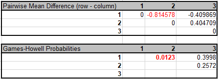
Click OK. The Pairwise Means Difference (Means
Matrix) and Games-Howell Probability results are:
The significant Games-Howell Probability values above have not
changed as compared to Welch Pairwise, but note that they are larger to compensate for
the family-wise error rate:
Note also that the 1 2 Games-Howell probability is smaller than
the Bonferroni corrected value = .0045 * 3 = .0135, so more powerful than Bonferroni.
The difference in power between Games-Howell and Bonferroni becomes more prominent with
a larger number of groups, so
Bonferroni is not included as an option.
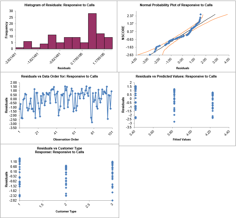
Click the Welch Residuals sheet tab to display the
Residual Plots:
Residuals are the unexplained variation from the ANOVA model
(Actual Predicted or Fitted values). Note that the residuals are not normally
distributed - as expected from the assumptions report - but like the regular ANOVA,
Welch's ANOVA is quite robust to the
assumption of normality. Also, as expected from Levene's test for equal variances, the
variability for Type 2 is less than Type 1, but Welchs ANOVA is robust to the
assumption of equal variances, so we can trust that the P-Values are valid.