DiscoverSim Case Studies
Case Study 8 — Optimization of Yield for 5 Factor Definitive Screening Design
Introduction: Optimization of Yield for 5 Factor Definitive Screening Design
This case study is adapted from Anderson et al., "Monte Carlo Simulation Experiments for Engineering Optimisation." See Case Study 8 References. A 5 Factor, Three Level, 13 Run Definitive Screening Design (DSD) was used to characterize the Yield of a chemical process. As noted in the paper, when there are only three or fewer active main effects, DSDs allow a full response surface model with two-factor interactions and quadratic terms to be modelled. See the SigmaXL Workbook for further details on Definitive Screening Designs.
The goal of the experiment is to maximize the Yield, with a lower specification limit = 75. A Yield value below 75 is a defect.
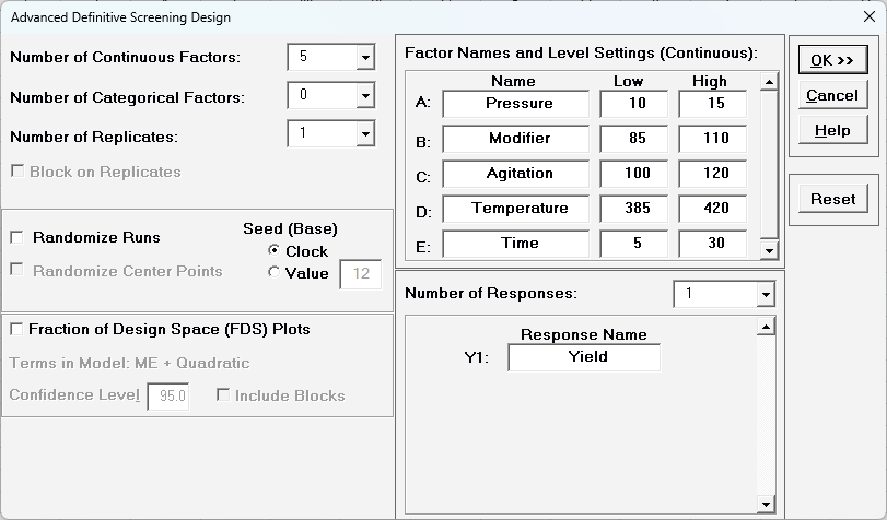
The factor names and level settings are given as:
Pressure: 10 — 15
Modifier: 85 — 110
Agitation: 100 — 120
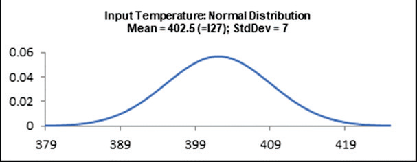
Temperature: 385 — 420
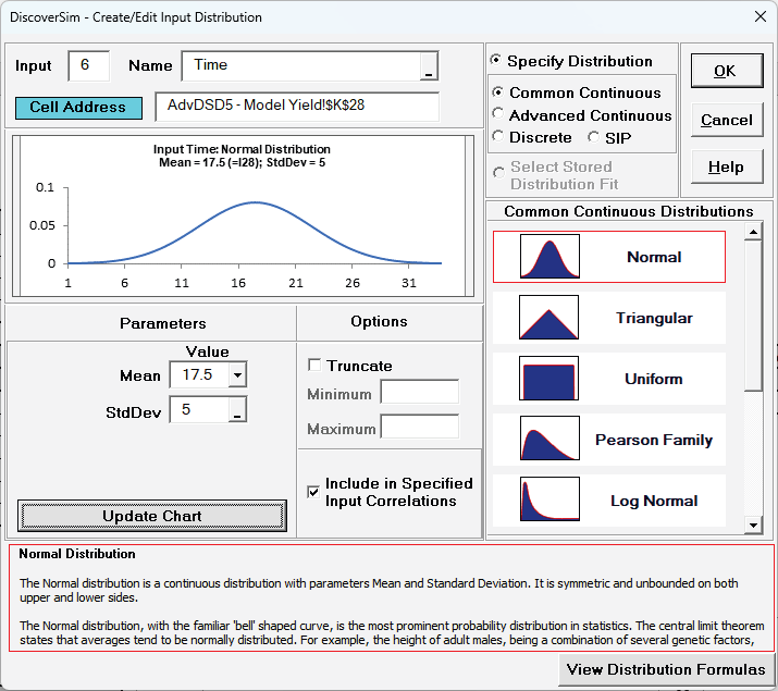
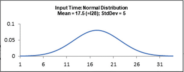
Time: 5 — 30
The experimental runs were randomized, but presented in standard order.
For Monte Carlo simulation of the significant factor inputs, a Normal Distribution was used with Mean initially at the nominal mid-point settings and Standard Deviation = Factor Range/5.
Note that the DSD design produced in SigmaXL is not identical to the one given in the paper (as produced by JMP software), but the design properties are identical. As a result, the Yield values given in the paper are not used, but estimated by simulation.
This is similar to Case Study 4 - Catapult Variation Reduction, where we are looking for settings that will minimize the transmitted variation.
Summary of DiscoverSim Features Demonstrated in Case Study 8:
|
- Create and Analyze a Definitive Screening Design in SigmaXL
- Convert SigmaXL Regression/DOE Model
- Create Continuous Input Distributions and Controls
- Add Model Error Term
- Run Simulation at Nominal Settings
- Optimization/Simulation: Maximize the Mean Yield
- Optimization/Simulation: Maximize PpL to Minimize Defects
|
Optimization of Yield for 5 Factor Definitive Screening Design
- We will begin with the creation of the 5 Continuous Factor DSD in SigmaXL. Click SigmaXL > Design of Experiments > Advanced Design of Experiments: Definitive Screening > Definitive Screening Designs. Select Number of Continuous Factors = 5, uncheck Randomize Runs and Fraction of Design Space (FDS) Plots. Enter the Factor Names and Level Settings and Response Name as shown.
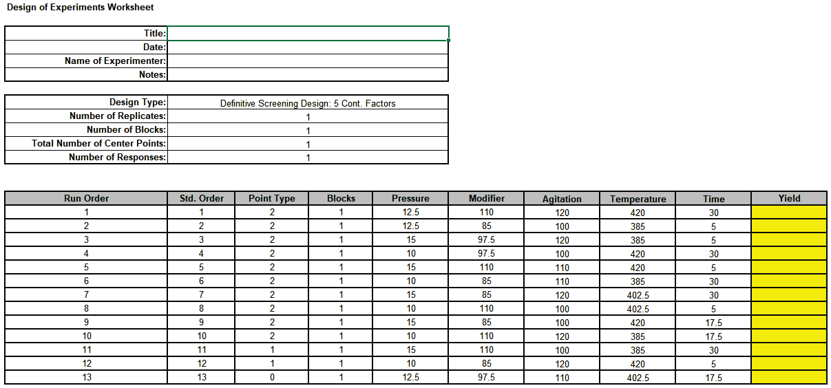
- Click OK. The Definitive Screening Design Worksheet is given as:
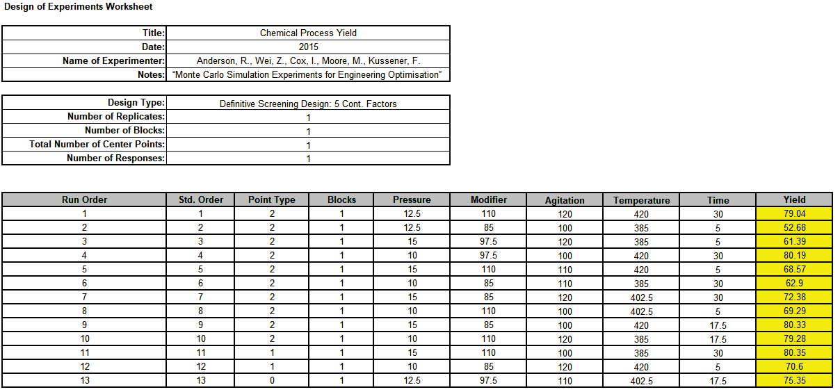
- Open the file Chemical Process Yield Anderson Five Factor DSD.xlsx. This has the design worksheet populated with Yield values.
- Click SigmaXL > Design of Experiments > Advanced Design of Experiments: Definitive Screening > Analyze Definitive Screening Design.
- Select Response and Model Terms as shown with Term Generator as ME + 2-Way Interactions + Quadratic. Click Select All >>. Check Residual Plots. Uncheck Main Effects Plots.
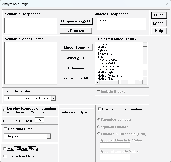
- There are more terms in the model than runs in the design so we will use Stepwise Forward Selection. Click
Advanced Options. Check Stepwise/Best Subsets Regression, select
Forward Selection, with Criterion AICc.
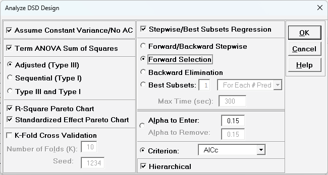
Alternatively, Best Subsets can be used for a more thorough evaluation of possible models, but we will not do so here. See the SigmaXL Workbook for more information on Advanced Options for Regression models.
- Click OK. Click OK.
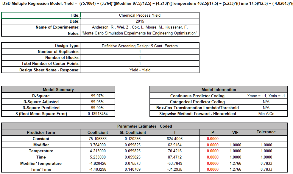
The final model from Stepwise Forward Selection matches the one given in the paper. R-Square, R-Square Adjusted and R-Square Predicted are all excellent. All terms are significant, VIF scores are close to 1 and the Residuals (Sheet
DSD — Residuals Yield) look good with no obvious non-normality, outliers or patterns.
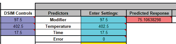
- The Predicted Response Calculator is given as:

- Click on Cell L26 to view the Excel formula which uses Range Names for the Factor Settings:
= (75.1063829787234) + (3.76400000000001)*((_Modifier_-97.5)/12.5) + (4.21300000000001)*((_Temperature_-402.5)/17.5) + (5.23300000000001)*((_Time_-17.5)/12.5) + (-4.82042553191488)*((_Modifier_-97.5)/12.5)*((_Temperature_-402.5)/17.5) + (-4.40329787234043)*((_Time_-17.5)/12.5)*((_Time_-17.5)/12.5)
- Now we will make a copy of this model in a new workbook for further analysis in DiscoverSim. Click on Sheet DSD � Model Yield. Click DiscoverSim > Help > Convert SigmaXL Regression/DOE Model.
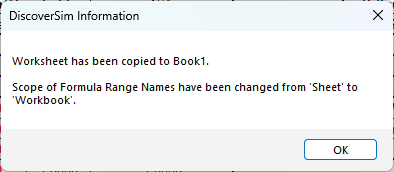
This conversion is necessary because the Predicted Response Calculator in the SigmaXL model uses Range Names that are scoped to the Sheet, but DiscoverSim requires Range Names that are scoped to the Workbook.
- Click OK. Rename the file (File > Save As) to Chemical Process Yield Anderson DSIM.xlsx.
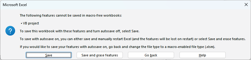
Click Save to keep the VBA script which computes the SE/CI/PI in the Predicted Response Calculator and the Optimize & Contour/Surface Plot button code. Note that these will not be used by DiscoverSim, so can also be erased if desired.
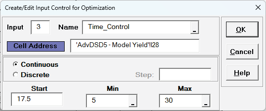
- First, we will add DiscoverSim Controls. Click on cell I26. Select Control:
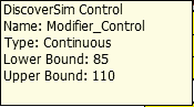
- For Name enter Modifier_Control. Select Continuous. For Start enter the mid-point value = 97.5. Set the Min value = 85 and the Max value = 110 as shown.

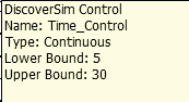
- Click OK. Hover the cursor on cell I26 to view the comment displaying the input control settings:
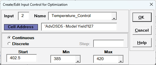
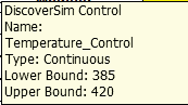
- Repeat steps 12-14 at cell I27 and I28 to create controls for Temperature and Time.
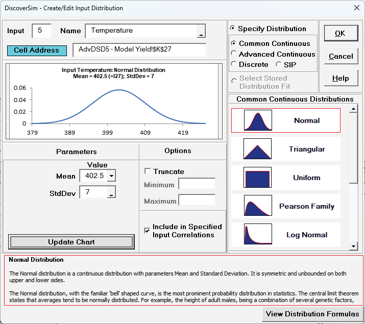
- Next, we will create the Input Distributions. Click on cell K26 to specify the Input Distribution for Modifier. Select DiscoverSim > Input Distribution:

- We will use the default Normal Distribution. For Name, enter Modifier.
- Click the Mean parameter cell reference
 and specify cell I26, the Modifier_Control with the Nominal Start Value = 97.5.
- Enter StdDev = 5. As noted earlier, the Monte Carlo simulation standard deviation used in the paper is: (High — Low)/5.
- Click Update Chart to view the Normal Distribution as shown:

- Click OK. Hover the cursor on cell K26 to view the DiscoverSim graphical comment showing the distribution and parameter values:
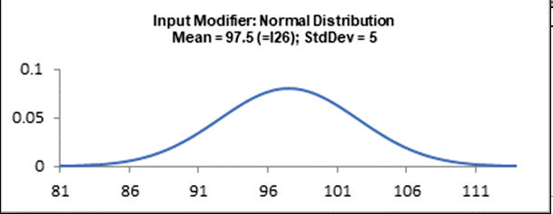
- Repeat Steps 16 — 21 at cells K27 and K28 to create Input Distributions for Temperature and Time:
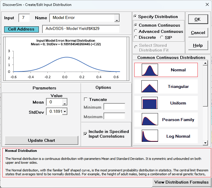
- Repeat Steps 16 — 21 at cell K29 to create an Input Distribution for Model Error. In this case, set Mean = 0 and StdDev references cell C22, the Model S (Root Mean Square Error):
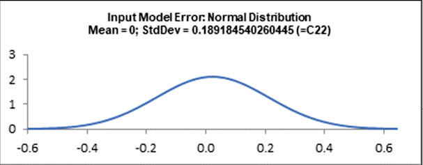
- Next, we will add the Model Error to the Predicted Response formula. Click on cell
L26. In the Formula Bar add +K29 as shown.
= (75.1063829787234) + (3.76400000000001)*((_Modifier_-97.5)/12.5) + (4.21300000000001)*((_Temperature_-402.5)/17.5) + (5.23300000000001)*((_Time_-17.5)/12.5) + (-4.82042553191488)*((_Modifier_-97.5)/12.5)*((_Temperature_-402.5)/17.5) + (-4.40329787234043)*((_Time_-17.5)/12.5)*((_Time_-17.5)/12.5)+K29
- Now we will specify the predicted response formula as the output. With the cursor on cell L26, select DiscoverSim > Output Response:

- Enter the output Name as "Yield" and the LSL = 75. Set Output Goal to Maximize.
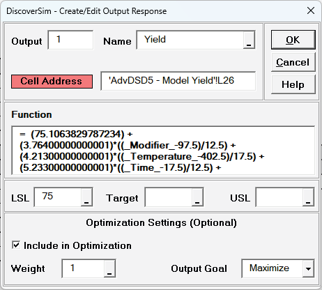
Note that setting Output Goal to Maximize is for information purposes and is not strictly necessary as it would only be used in a Multiple Response Optimization.
- Click OK.
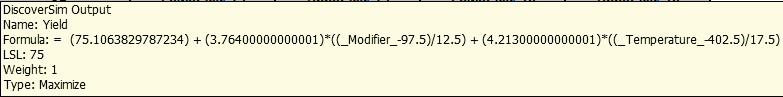
- Hover the cursor on cell L26 to view the DiscoverSim Output information.
- Save the file. The completed model can optionally be labelled and formatted as shown:
- We are now ready to perform a simulation run. This is our baseline, after which we will run an optimization to maximize the Yield and compare the results.
- Select DiscoverSim > Run Simulation:

- Select Seed Value and enter "12" as shown, in order to replicate the simulation results given below.
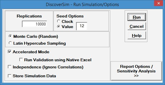
- Click Run.
- The DiscoverSim Output Report shows a Histogram, Descriptive Statistics, Normality Tests, Process Capability and Performance Indices:
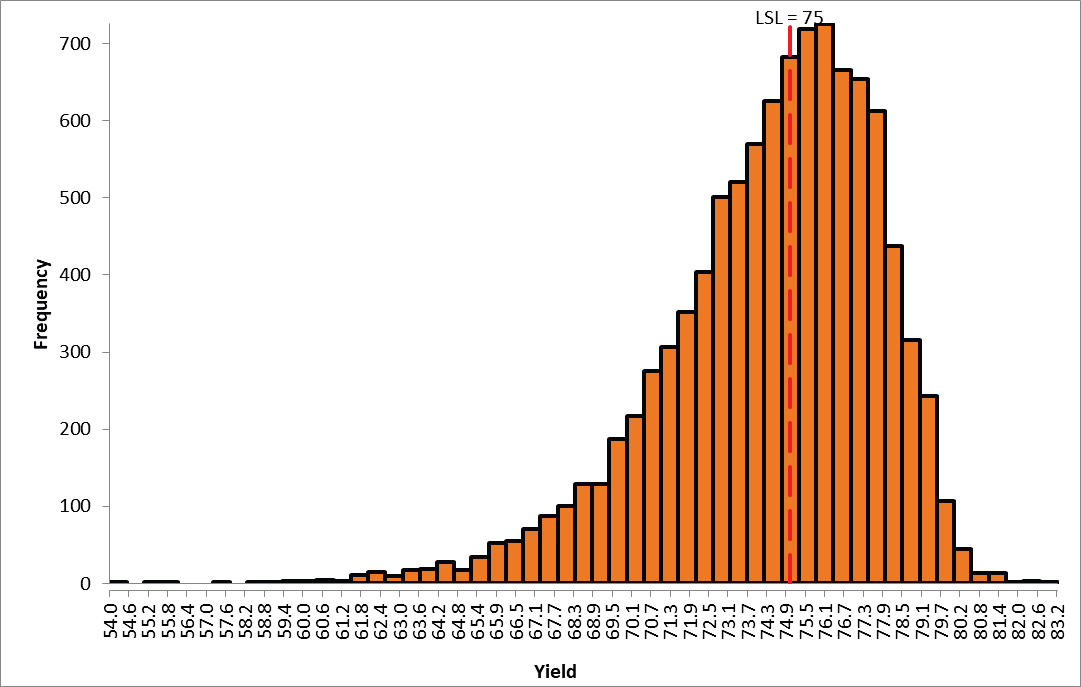
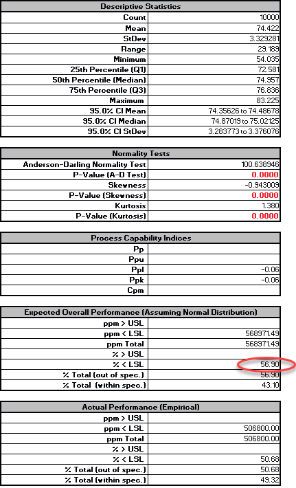
- From the histogram and capability report we see that the output Yield is not capable of meeting the specification requirements using the baseline values. Since the response data is not normal, we will use the Actual Performance (Empirical) for evaluation. The % 〈 LSL = 50.7, which is unacceptable.
- Now we will optimize the process by maximizing the Mean Yield. Select DiscoverSim > Run Optimization:

- Select "Maximize" for Optimization Goal, "Weighted Sum" for Multiple Output Metric and "Mean" for Statistic. Select Hybrid. Select Seed Value and enter "12" in order to replicate the optimization results given below. All other settings will be the defaults as shown:
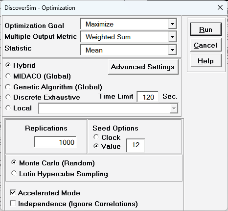
- Click Run. This optimization will take approximately 2 minutes. To save time, you may wish to click the Interrupt button after a few seconds.
- The final optimal parameter values are given as:
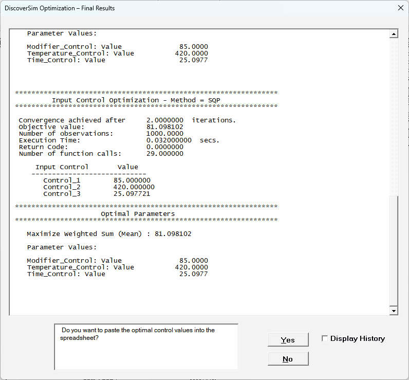
- Click Yes to paste the optimal control values into model cells I26 to I28.
- Select DiscoverSim > Run Simulation:

- Select Seed Value and enter "12" as shown, in order to replicate the simulation results given below.

- Click Run.
- The DiscoverSim Output Report shows a Histogram, Descriptive Statistics, Normality Tests, Process Capability and Performance Indices:
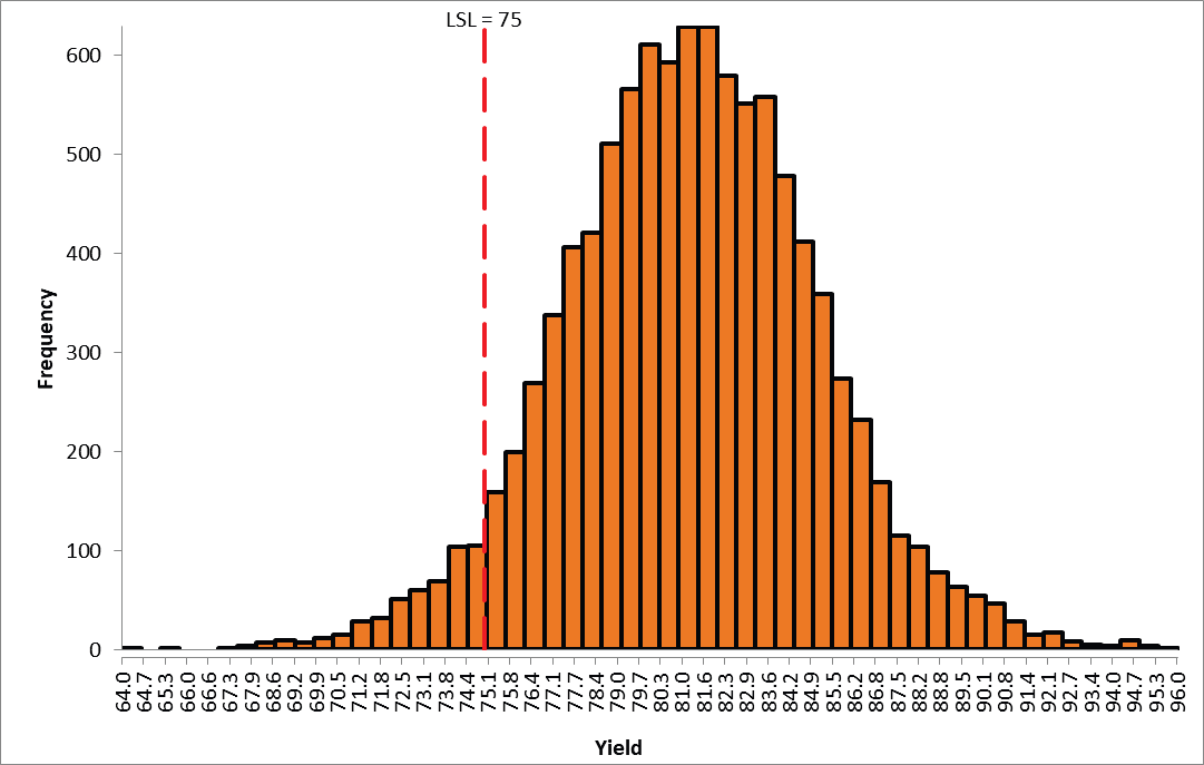
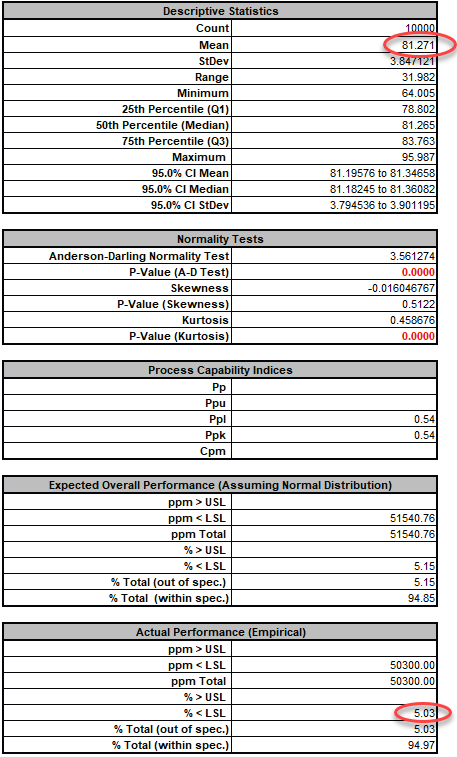
- From the histogram and capability report, we see that the output Yield Mean has improved from 74.4 to 81.3. Since the response data is not normal, we will use the Actual Performance (Empirical) for evaluation. The % 〈 LSL has been dramatically reduced from 50.68 to 5.03.
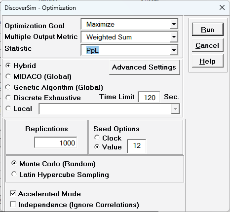
- Now we will further optimize the process by maximizing the Process Capability Index PpL. Select DiscoverSim > Run Optimization:

- Select "Maximize" for Optimization Goal, "Weighted Sum" for Multiple Output Metric and "PpL" for Statistic. Select Hybrid. Select Seed Value and enter "12" in order to replicate the optimization results given below. All other settings will be the defaults as shown:
- Click Run. This optimization will take approximately 2-3 minutes. To save time, you may wish to click the Interrupt button after a few seconds.
- The final optimal parameter values are given as:
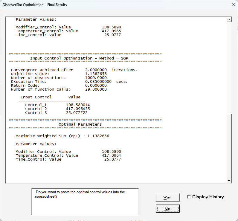
- Click Yes to paste the optimal control values into model cells I26 to I28.
- Select DiscoverSim > Run Simulation:

- Select Seed Value and enter "12" as shown, in order to replicate the simulation results given below.

- Click Run.
- The DiscoverSim Output Report shows a Histogram, Descriptive Statistics, Normality Tests, Process Capability and Performance Indices:
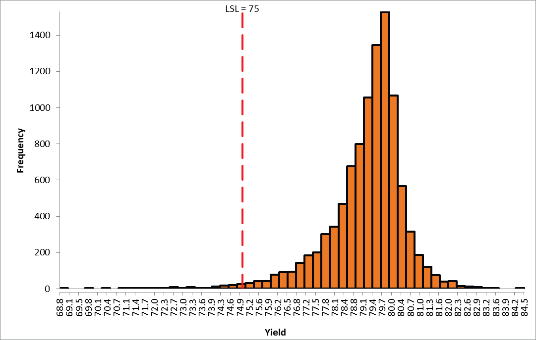
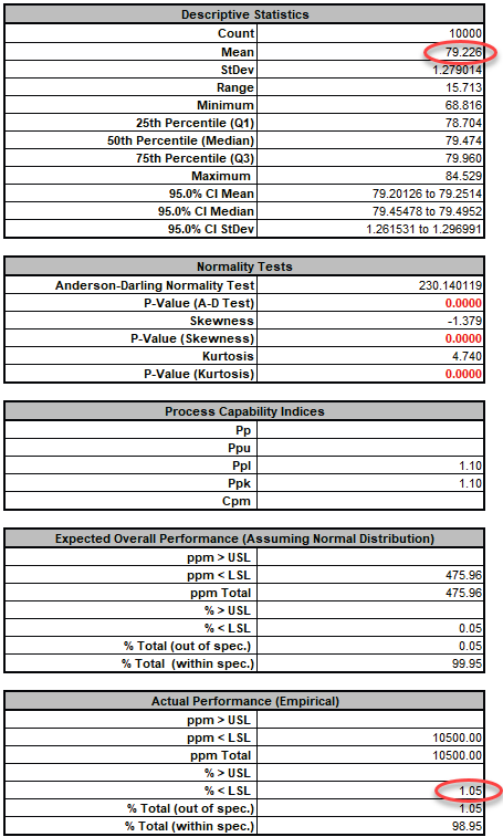
- From the histogram and capability report we see that the output Yield Mean has decreased slightly from 81.3 to 79.2, but the StDev has been dramatically reduced from 3.85 to 1.28, and the objective function process capability index PpL has increased from 0.54 to 1.1. The Actual Performance (Empirical) % 〈 LSL has been further reduced from 5.03 to 1.05.
- These results are similar to those reported in the paper. DiscoverSim was able to find the settings that minimize the transmitted variation, making the process robust and reduce the defect rate.
Case Study 8: References
Anderson, R., Wei, Z., Cox, I., Moore, M., Kussener, F. (2015). "Monte Carlo Simulation Experiments for Engineering Optimisation," Studies in Engineering and Technology, Vol. 2, No. 1, Redfame Publishing, https://redfame.com/journal/index.php/set/article/view/901.


