DiscoverSim Case Studies

DiscoverSim Case Study 6 — Multiple Response Optimization and Practical Tolerance Design

Introduction: Optimizing Low Pass RC Filter

---

The passive low pass RC (Resistor Capacitor) filter network shown below has been analyzed in several papers (see Case Study 6 References ) and will be used to demonstrate how DiscoverSim allows you to easily solve the difficult problems of multiple response optimization for parameter design and practical tolerance design.

The design approaches presented in the reference papers and books include: Axiomatic Design (Suh, El-Haik), Taguchi Methods (Filippone), Analytical Design for Six Sigma (Ferryanto), and Integrated Parameter and Tolerance Design using Factorial Design of Experiments and Loss Function (Feng).

Acknowledgements and thanks to Dr. Eric Maass and Andrew Sleeper for their valuable feedback on this case study.

The RC filter network to be designed (C, R1 and R2) suppresses the high-frequency carrier signal and passes only the desired low-frequency displacement signal from the strain-gage transducer to the recorder with a galvanometer/light-beam deflection indicator (El-Haik, Feng). Light beam galvanometers have been replaced with digital oscilloscopes, but they still have practical application today in laser scanning systems.

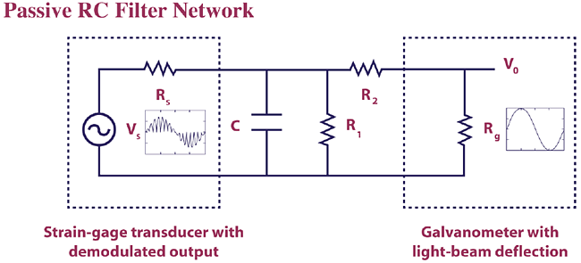
Vs is the demodulated transducer voltage and Rs is the transducer resistance (impedance). Rg is the galvanometer terminal resistance. Vo is the galvanometer output voltage which produces the deflection displacement. One of the output responses of interest, galvanometer full scale deflection D, is a function of Vo, Rg, and the galvanometer sensitivity Gs. The values for Vs, Rs, Rg, and Gs are determined by the transducer and galvanometer vendors and are therefore considered as noise factors. We will use the nominal and tolerance values given by Feng and Filippone for the noise factors: Vs = 15 mV; Rs = 120 ohms; Rg = 84 ohms; Gs = 0.56364 mA/inch. All tolerance values are 0.15%. We will model these noise factors using a normal distribution with mean set to the nominal value and standard deviation calculated as nominal*(tolerance/100)/3 = nominal*0.0015/3.

Capacitor C, and resistors R1, R2 are the components of the passive filter network. These are the design control factors of interest in this study. The mean values for C, R1, and R2 will be varied using parameter design optimization to meet the required output specifications with minimal variation. Tolerances on these components are also noise factors that contribute to variability in the output but we can select those tolerance values that are required to give us the desired performance. The starting nominal and tolerance values will be those given in Feng and Filippone: C = 257 µF, R1 = 1060 ohms, and R2 = 464 ohms with tolerance = 5% for each. As with the noise factors, we will model the control factors using a normal distribution with mean initially set to the nominal value and standard deviation initially set to nominal*(tolerance/100)/3 = nominal*0.05/3.

The output responses of interest are full scale deflection D and filter cut-off frequency F. The equations (derived from Kirchhoff's Current Law) are given as:

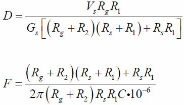
Note: Resistors R₁ and R₂ affect both output responses, and capacitor C only affects the cut-off frequency F.

The target value for Deflection D is 3.0 inches. We will use 1% as the tolerance for D so the lower specification limit LSLD = 2.97 and upper specification limit USLD = 3.03. The target value for Filter Cut-Off Frequency F is 6.84 Hz. We will use 5% as the tolerance for F so LSLF = 6.498 and USLF = 7.182. Process Capability indices will be used to measure the quality of each output response, but optimization will be performed by minimizing the multiple output metric Weighted Sum of Mean Squared Error (MSE), also known as the loss function:

MSE (Loss) = WeightD[(MeanD − TargetD)2 + StdDevD2] + WeightF[(MeanF − TargetF)2 + StdDevF2]

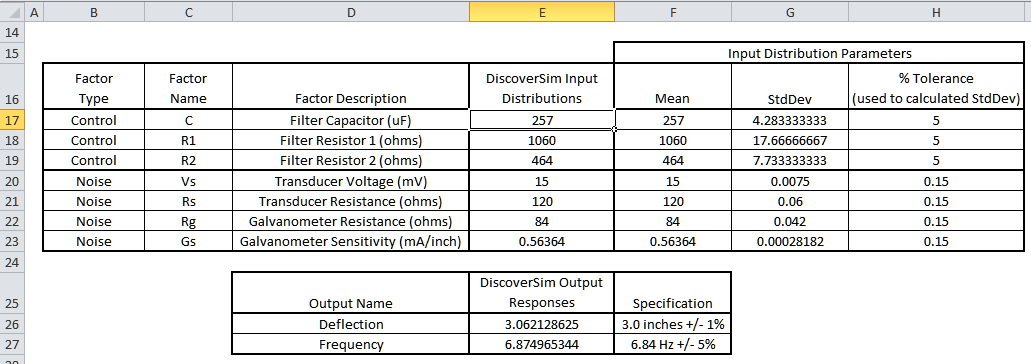
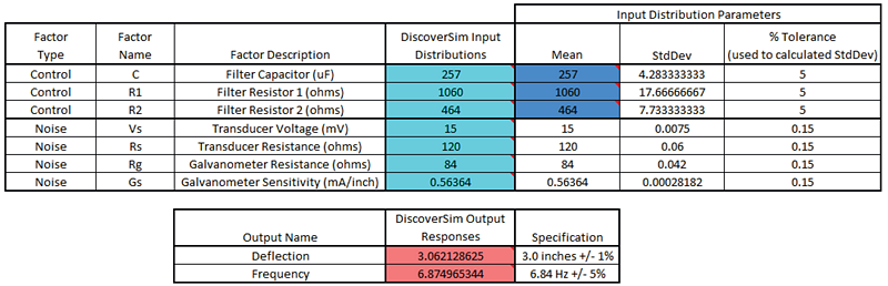
The control and noise factor settings are summarized in the table below:

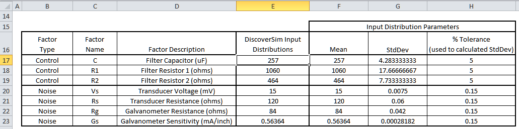
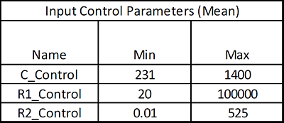
The minimum and maximum mean values used for parameter optimization of the control factors are the values from Filippone for the Taguchi Inner Array:

(Note that if we did not have the above nominal mean values for control factors available as starting values, we would use the mid-point of the minimum/maximum to start the optimization. The final optimization result would be the same in either case because the optimizer is global not local.)

We will also consider standard component availability and cost in this case study (source: electronic component supplier www.mouser.com ). One practical concern will be the capacitor. Capacitors larger than 230 µF will typically be electrolytic with a 20% tolerance or more, so specifying a tolerance of 5% or less will significantly increase the component cost.

In this study we will use DiscoverSim to help us answer the following questions:

• What are the predicted process capability indices with the published nominal settings?


• What are the predicted process capability indices after parameter optimization? How do they compare to the baseline results above?


• What are the key control factors (Xs) that influence Deflection D and Frequency F?


• What standard components are available that are close to the optimal values obtained from parameter design?


• What tolerances are available for those standard components? Can we minimize the component cost and achieve a Six Sigma quality design?

Summary of DiscoverSim Features Demonstrated in Case Study 6:

Create Input Distributions (Continuous Normal) DiscoverSim Copy/Paste Cell Run Simulation with Sensitivity Chart of Correlation Coefficients Create Continuous Input Controls for Parameter Optimization Run Optimization for Multiple Outputs

Multiple Response Optimization and Practical Tolerance Design of Low Pass RC Filter with DiscoverSim

1. Open the workbook Passive RC Filter Design. DiscoverSim Input Distributions will simulate the variability in control and noise component tolerances. The Normal Distribution (as used in the reference papers) will be specified in cells E17 to E23. The mean values are specified in cells F17 to F23. The standard deviation values are calculated in cells G17 to G23 as discussed above to model the component tolerances, specified in cells H17 to H23. Input Controls will be added to cells F17 to F19 which will vary the mean for the control factors C, R1 and R2 in optimization. The outputs, Deflection and Frequency, will be specified in cells E26 and E27 using the formulas given above.
   
   


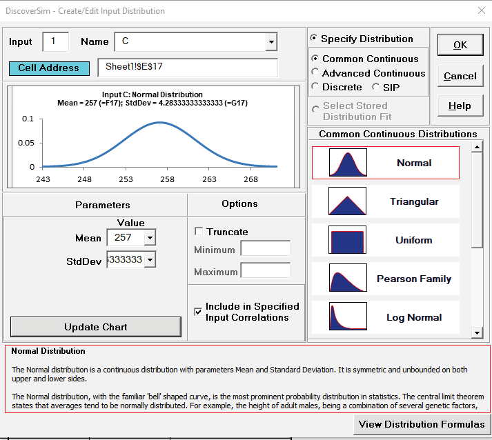
2. Click on cell E17 to specify the Input Distribution for the Capacitor C. Select DiscoverSim > Input Distribution:
   
   


3. We will use the default Normal Distribution.


4. Click input Name cell reference and specify cell C17 containing the input name C. After specifying a cell reference, the dropdown symbol changes from to .


5. Click the Mean parameter cell reference and specify cell F17 containing the mean parameter value = 257.


6. Click the StdDev parameter cell reference and specify cell G17 containing the standard deviation parameter value = Mean * (Tolerance/100)/3 = (257 * .05)/3 = 4.283.


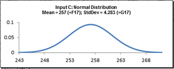
7. Click Update Chart to view the normal distribution as shown:
   
   


8. Click OK. Hover the cursor on cell E17 to view the DiscoverSim graphical comment showing the distribution and parameter values:
   
   


9. Click on cell E17. Click the DiscoverSim Copy Cell menu button (Do not use Excel's Copy it will not work!).


10. Select cells E18:E23. Click the DiscoverSim Paste Cell menu button (Do not use Excel's Paste it will not work!).


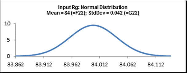
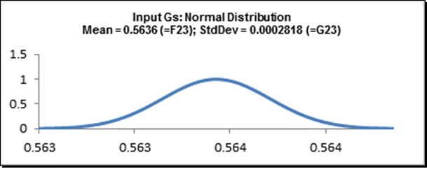
11. Review the input comments in cells E18 to E23:
    
    Cell E18:
    
    
    
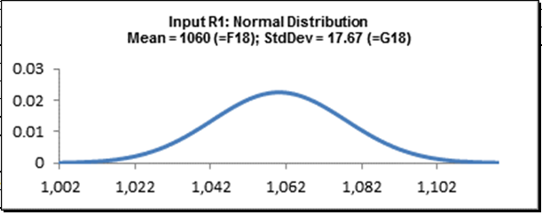
    Cell E19:
    
    
    
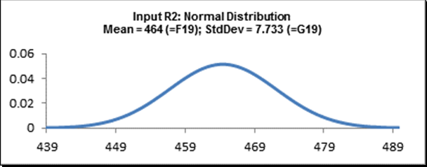
    Cell E20:
    
    
    
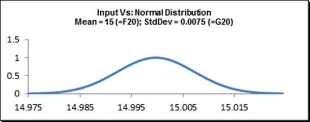
    Cell E21:
    
    
    
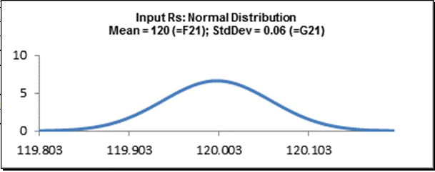
    Cell E22:
    
    
    
    Cell E23:
    
    


12. Now we will specify the outputs. Click on cell E26. Note that the cell contains the Excel formula for Deflection:
    =(_Vs*_Rg*_R1)/(_Gs*((_R2+_Rg)*(_Rs+_R1)+_Rs*_R1)).
    Excel range names are used rather than cell addresses to simplify interpretation.


13. Select DiscoverSim > Output Response:
    
    


14. Enter the output Name as Deflection. Enter the Lower Specification Limit (LSL) as 2.97, Target as 3, and Upper Specification Limit (USL) as 3.03. Weight = 1 and Output Goal should be Target.
    
    
    
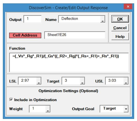
    Click OK.


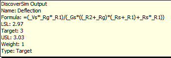
15. Hover the cursor on cell E26 to view the DiscoverSim Output information.
    
    


16. Click on cell E27. Note that the cell contains the Excel formula for Frequency:
    =((_R2+_Rg)*(_Rs+_R1)+_Rs*_R1)/(2*PI()*(_R2+_Rg)*_R1*_Rs*_C*0.000001)


17. Select DiscoverSim > Output Response:
    
    


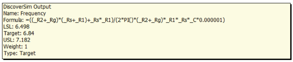
18. Enter the output Name as Frequency. Enter the Lower Specification Limit (LSL) as 6.498, Target as 6.84, and Upper Specification Limit (USL) as 7.182. Weight = 1 and Output Goal should be Target.
    
    
    
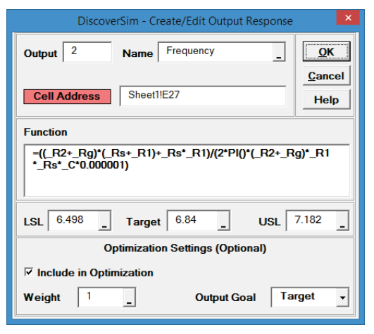
    Click OK.


19. Hover the cursor on cell E27 to view the DiscoverSim Output information.
    
    


20. Now we are ready to perform a simulation run. This is our baseline, after which we will run parameter optimization and compare results. We will also perform a Sensitivity Analysis after optimization.


21. Select DiscoverSim > Run Simulation:
    
    


22. Select Seed Value and enter 12 as shown, in order to replicate the simulation results given below.
    
    
    
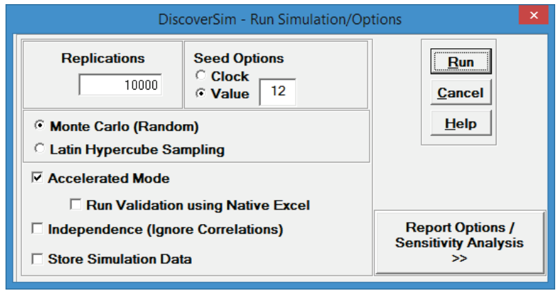
    Click Run.


23. The DiscoverSim Output Report shows a histogram, descriptive statistics and process capability indices for each output.
    
    Deflection Report:
    
    
    
    
    
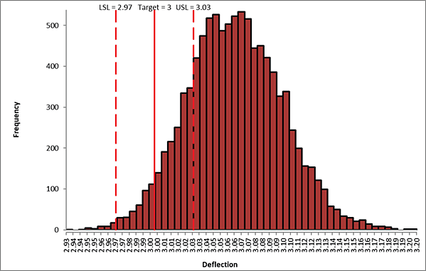
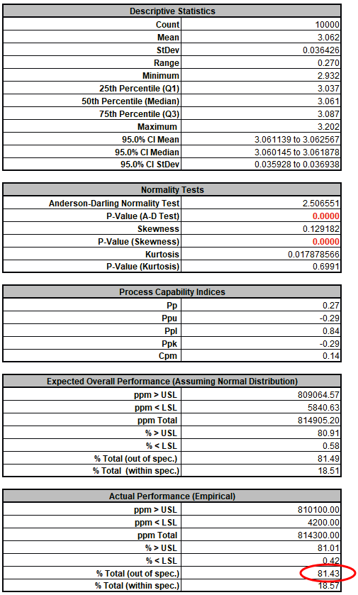
    From the histogram and capability report we see that the output Deflection is not capable of meeting the specification requirements using the baseline values. The process mean is off target and the variation due to component tolerance is unacceptably large. We expect that 81.4% of the units would fail this requirement, so we must improve the design to center the mean and reduce the variation of Deflection, while simultaneously satisfying the Frequency requirement.
    
    Frequency Report:
    
    
    
    
    
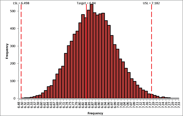
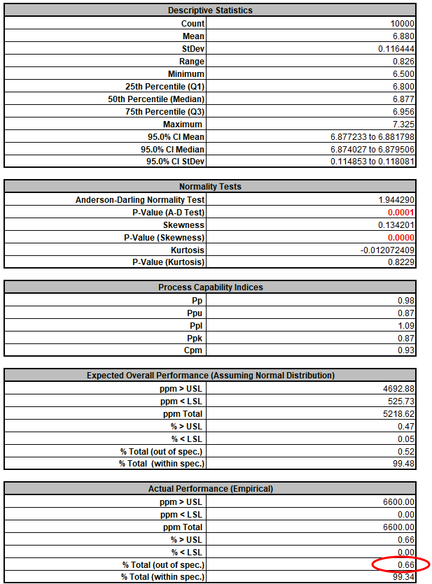
    From the histogram and capability report we see that the output Frequency is slightly off target and just capable of meeting the specification requirements using the baseline values. We expect that 0.66% of the units would fail this requirement, so if possible we should improve the design to reduce the variation of Frequency while simultaneously improving Deflection.


24. In order to run optimization, we will need to add the Input Controls in cells F17 to F19. Select Sheet1. The Input Control parameters (min/max) are shown below (from Filippone):
    
    
    
    These controls will vary the nominal mean values for C, R1 and R2. The standard deviation will be recalculated with each optimization iteration, so that a 5% tolerance is preserved (see above for formula).


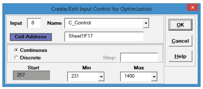
25. Click on cell F17. Select Control:
    
    


26. Click Input Name cell reference and specify cell J17 containing the input control name C_Control.


27. Click the Min value cell reference and specify cell K17 containing the minimum optimization boundary value = 231.


28. Click the Max value cell reference and specify cell L17 containing the maximum optimization boundary value = 1400:
    
    


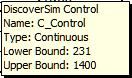
29. Click OK. Hover the cursor on cell F17 to view the comment displaying the input control settings:
    
    


30. Click on cell F17. Click the DiscoverSim Copy Cell menu button (Do not use Excel's Copy it will not work!).


31. Select cells F18:F19. Click the DiscoverSim Paste Cell menu button (Do not use Excel's Paste it will not work!).


32. Review the Input Control comments in cells F17 to F19.


33. The completed model is shown below:
    
    


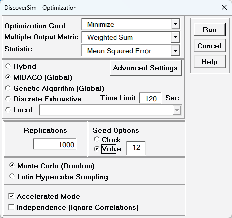
34. Now we are ready to perform the optimization. Select DiscoverSim > Run Optimization:
    
    


35. Select "Minimize" for Optimization Goal, "Weighted Sum" for Multiple Output Metric and "Mean Squared Error" for Statistic. Select MIDACO (Global). Select Seed Value and enter 12, in order to replicate the optimization results given below. Set Replications to 1000 to reduce the optimization time. All other settings will be default as shown:
    
    
    
    Mean Squared Error, also known as a Loss Function, is discussed above:
    
    MSE (Loss) = Weight_D[(Mean_D − Target_D)² + StdDev_D²] + Weight_F[(Mean_F − Target_F)² + StdDev_F²]
    
    We want both the Deflection and Frequency outputs to be on target with minimal variation. The weights were set when the outputs were created and are the same for each output (= 1).
    
    We will use the MIDACO optimization method which is powerful to solve complex optimization problems.


36. Click Run. This optimization will take approximately 2 minutes.


37. The final optimal parameter values are given as:
    
    


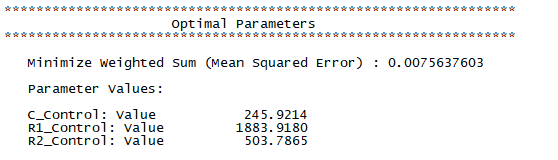
38. You are prompted to paste the optimal values into the spreadsheet:
    
    
    
    Click Yes. This replaces the nominal input control values with the new optimum values. Note that the displayed values for the input distributions at cells E17 to E19 are not overwritten, but when the simulation is run, the referenced mean and standard deviation given in F17 to G19 will be applied.


39. Select Run Simulation. Click Report Options/Sensitivity Analysis. Check Sensitivity Charts and Correlation Coefficients. Select Seed Value and enter 12, in order to replicate the simulation results given below. Click Run.


40. The DiscoverSim Output Report shows a histogram, descriptive statistics and process capability indices for each output.
    
    Deflection Report (after optimization):
    
    
    
    
    
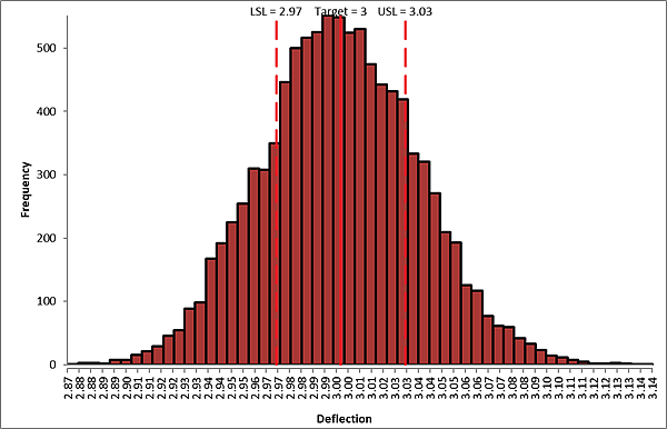
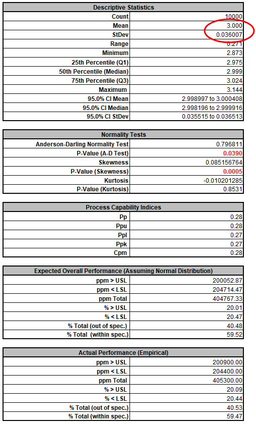
    From the histogram and capability report we see that the output Deflection is still not capable of meeting the specification requirements after optimization, however the mean is now on target (mean shifted from 3.062 to 3.000). The expected performance failure rate was reduced from 81.43% to 40.53% due to centering the mean. Since we only saw a slight reduction in the standard deviation (0.0364 to 0.0360), the component tolerances will need to be tightened. The sensitivity analysis will help us to focus on which components are critical and require tighter tolerances.
    
    Frequency Report (after optimization):
    
    
    
    
    
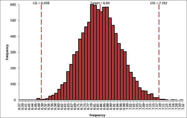
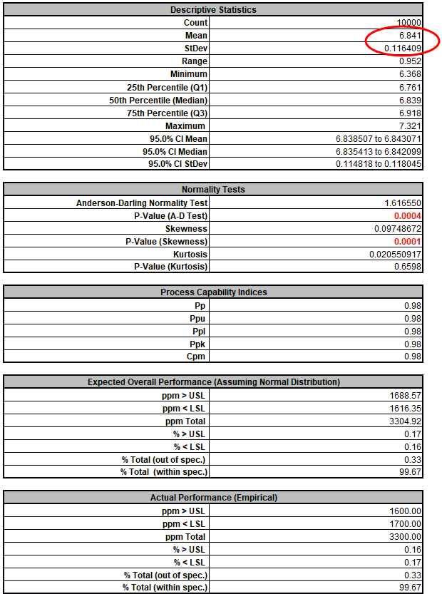
    From the histogram and capability report we see that the output Frequency after optimization is now on target (mean shifted from 6.880 to 6.841) but still just capable of meeting the specification. The actual performance failure rate was reduced from 0.66% to 0.33% due to centering the mean. Since we did not see a reduction in the standard deviation, the component tolerances will need to be tightened. As with Deflection, the sensitivity analysis will help us to focus on which components are critical and require tighter tolerances.


41. Click on the Sensitivity Correlations sheet:
    
    
    
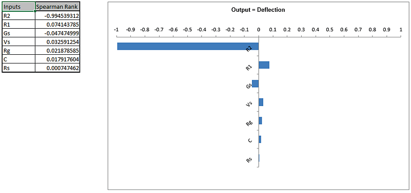
    Resistor R2 is the dominant component affecting Deflection. A search at the electronic component supplier www.mouser.com, shows that 510 ohm resistors ( watt axial) with a 5% tolerance or 1% tolerance, cost approximately $0.04 each (qty. 100 pricing); resistors with a 0.1% tolerance are $0.29 to $1.00 each. Since R2 has such a strong influence on the variability we will use 0.1% tolerance, even with the higher cost. Afterward, we will consider using 1% tolerance for R2 as a possible cost saving measure. Even though resistor R1 has negligible influence (on Deflection or Frequency below), we will use a 1% tolerance since the price is approximately the same as that of 5% tolerance resistors (5K ohms value).


42. Frequency Sensitivity Chart:
    
    
    
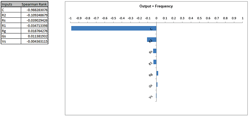
    Capacitor C is the dominant component affecting Frequency, followed by Resistor R2. Unfortunately, capacitors larger than 230 µF will typically be electrolytic with a 20% tolerance or more. Specifying a tolerance of 5% or less will significantly increase the component cost. Another issue is that the number of available capacitor standard values is very limited compared to that of resistors. We need to reduce the variability of Frequency so we will specify a 2% tolerance (electrolytic > 10V axial). The lowest cost option available to us in the 230 to 300 µF range is a Vishay 280 µF @2%, at $11.79 each (qty. 101). If this cost is unacceptable then we would need to use a 20% tolerance and relax the output specifications for Frequency or accept the lower process capability/higher defect rate. The cost for a 250 µF @20% is $1.84, qty. 100.


43. Now we will modify the control factor settings and rerun the optimization for practical tolerance design, starting with the fixed capacitor value of 280 µF @2% tolerance. The capacitor is selected first because of the limited selection for available capacitor standard values.


44. Enter the value 280 in control cell F17. Click on cell H17 and change the tolerance value to 2, resulting in a reduced standard deviation value in cell G17 for capacitor C.
    
    
    
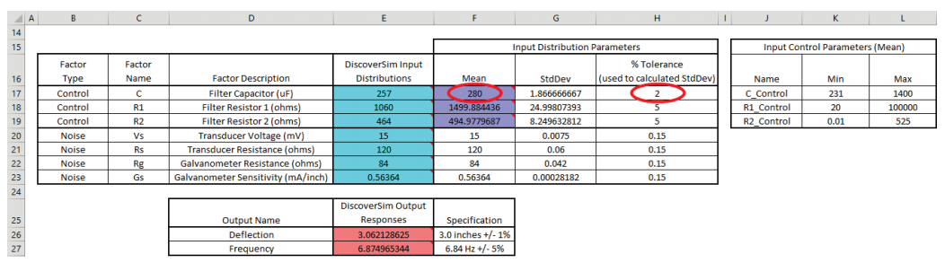
    Note: The original E17 cell value of 257 for input distribution C is not overwritten in the sheet display, but the referenced control value in F17, 280, will be used in simulation and further optimization.


45. Click on cell H18 and change the tolerance value to 1, resulting in a reduced standard deviation value in cell G18 for resistor R1.
    
    


46. Click on cell H19 and change the tolerance value to 0.1, resulting in a reduced standard deviation value in cell G19 for resistor R2.
    
    


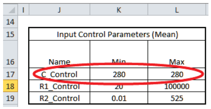
47. Enter the Input Control min/max values for C in cells K17 and L17 as 280. This fixes the C value so that it will not vary in optimization.
    
    


48. Now we are ready to perform the optimization. Select DiscoverSim > Run Optimization:
    
    


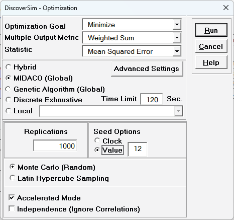
49. Select "Minimize" for Optimization Goal, "Weighted Sum" for Multiple Output Metric and "Mean Squared Error" for Statistic. Select MIDACO (Global). Select Seed Value and enter "12", in order to replicate the optimization results given below. Set Replications to 1000 to reduce the optimization time. All other settings will be default as shown:
    
    


50. Click Run. This optimization will take approximately 1 minute.


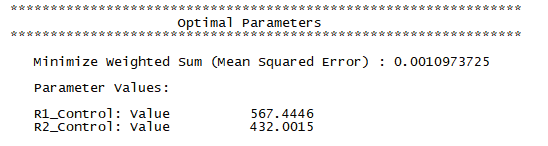
51. The final optimal parameter values are given as:
    
    


52. You are prompted to paste the optimal values into the spreadsheet:
    
    
    
    Click Yes. This replaces the nominal input control values with the new optimum values.


53. For R2 we will use a ¼ watt axial 432 ohm 0.1% tolerance resistor, available at a cost of $0.64 each (qty 100). Later we will consider using a 432 ohm 1% tolerance resistor as a possible cost saving measure since they are only $0.04 each (qty 100).


54. For R1, we will use a ¼ watt axial 565 ohm 1% tolerance resistor for R1, which is the closest available standard value to 566.8 ohms.


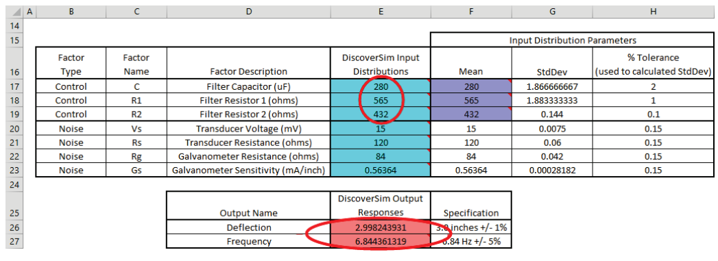
55. Enter the value 565 in control cell F18 for R1. The 1.0% tolerance specified in cell H18 does not change. Enter the value 432 in control cell F19 for R2. The 0.1% tolerance specified in cell H19 does not change.
    
    


56. It is not necessary to freeze the R1 and R2 min/max values since we are no longer running optimization.


57. Now type in the C, R1 and R2 values in the Input Distributions cells E17 to E19. Note that this is not required to run the simulation, but allows us to quickly check what the expected values will be for the outputs Deflection (at E26) and Frequency (at E27).
    
    


58. Now we are ready to perform the simulation. Select Run Simulation. Click Run.


59. The DiscoverSim Output Report shows a histogram, descriptive statistics and process capability indices for each output, and confirms that the RC design has dramatically improved:
    
    
    
    
    
    
    
    


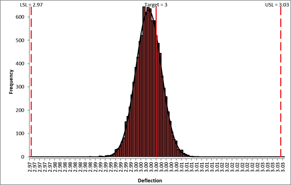
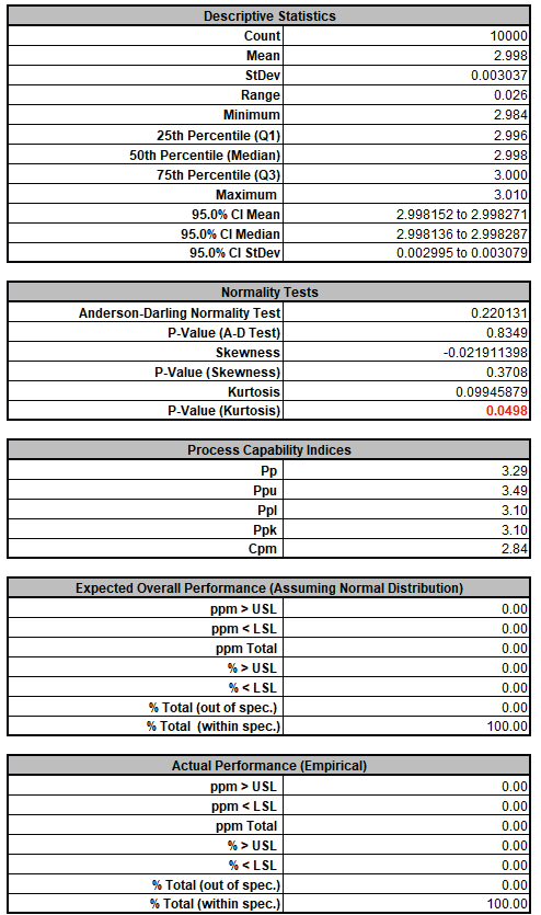
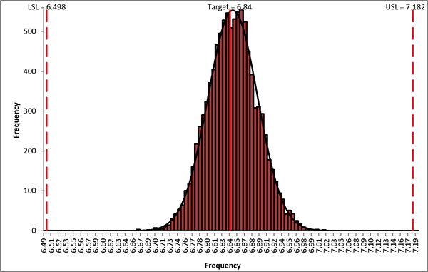
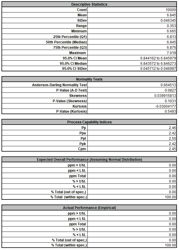
60. Now that we have achieved beyond Six Sigma quality for this design (Ppk > 1.5 for each output), we need to consider if we can relax the tolerance for R2 from 0.1% to 1%, thus reducing the component cost (from $0.64 each to $0.04 each in qty. 100).


61. Click on cell H19 and change the tolerance value from 0.1 to 1, resulting in an increased standard deviation value in cell G19 for resistor R2:
    
    


62. Now re-run the simulation. Select Run Simulation. Click Run.


63. The resulting simulation report for both outputs is shown below:
    
    
    
    
    
    
    

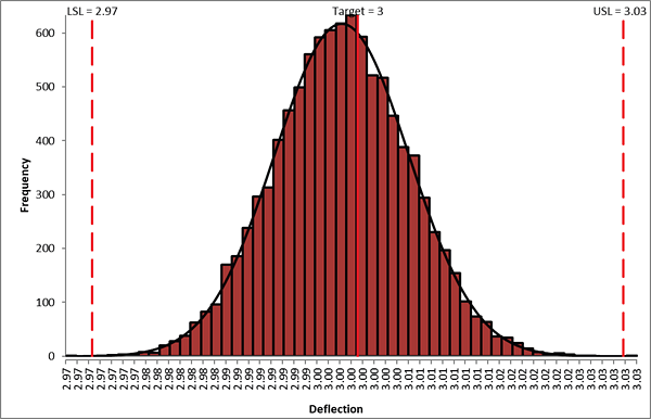
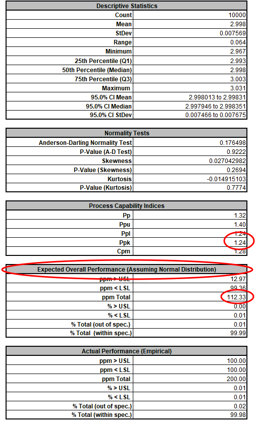
    As expected from our sensitivity analysis, we see that Ppk for Deflection has dropped from 3.10 to 1.24, and the expected ppm failure rate has increased from 0.0 to 112.33. (Here we also display the Sum of PPM report which includes the sum of ppm values for both Deflection and Frequency).

    
    
    
    
    
    
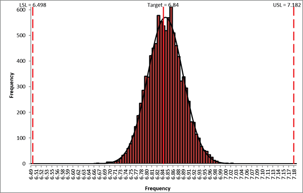
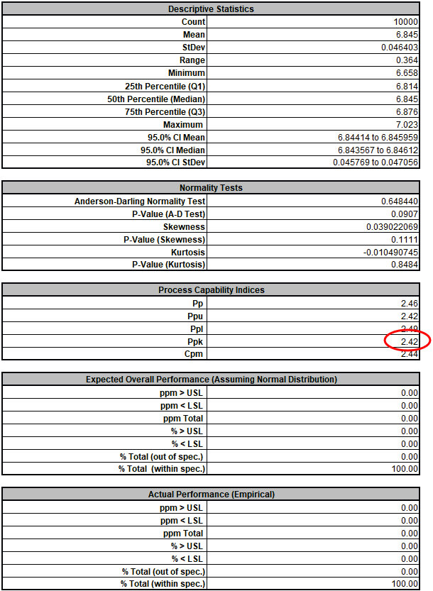
    We see that Ppk for Frequency has not changed from 2.42, so increasing the tolerance for R2 from 0.1% to 1% does not have any effect on Frequency.


64. Now that we have run both simulations, we see the trade-off between a difference in predicted ppm failure rate of 112 and a cost difference of 0.60 per unit, thus enabling us to make an informed decision of which tolerance to use for R2.


65. A similar analysis can be performed in the tolerance versus cost consideration for the capacitor.

Case Study 6: References

---

El-Haik, B.S. (2005) Axiomatic Quality: Integrating Axiomatic Design with Six-Sigma, Reliability, and Quality Engineering, Hoboken, N.J.: Wiley.

Feng, Q. (2008) An integrated method of parameter design and tolerance design for multiple criteria systems, Int. J. Computer Applications in Technology, Vol. 32, No. 2, pp.118—127.

Ferryanto, L. (2007) Analytical DFSS for multiple response products, Int. J. Six Sigma and Competitive Advantage, Vol. 3, No. 1, pp.13—32.

Filippone, S.F. (1989) Using Taguchi methods to apply the axioms of design, Robotics and Computer-Integrated Manufacturing, Vol. 6, pp.133—142.

Rinderle, J.R. (1982) Measures of Functional Coupling in Design, Thesis (Ph.D.) — Massachusetts Institute of Technology, Dept. of Mechanical Engineering.

Suh, N.P. (1990) The Principles of Design. New York, NY: Oxford Press.