Introduction: Optimizing Shutoff Valve Spring Force
This is an example of DiscoverSim stochastic optimization for robust new product design,
adapted from:
Sleeper, Andrew (2006), Design for Six Sigma Statistics: 59 Tools for Diagnosing and Solving
Problems in DFSS Initiatives, NY, McGraw-Hill, pp. 782-789.
Sleeper, Andrew, Accelerating Product Development with Simulation and Stochastic
Optimization
This example is used with permission of the author.
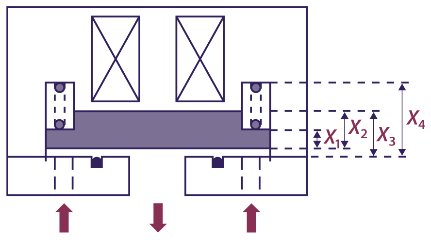
The figure below is a simplified cross-sectional view of a solenoid-operated gas shutoff
valve:
The arrows at the bottom of the figure indicate the direction of gas flow. A solenoid holds
the plate (shaded) open when energized. When the solenoid is not energized, the spring
pushes the plate down to shut off gas flow. If the spring force is too high, the valve will
not open or stay open. If the spring force is too low, the valve can be opened by the inlet
gas pressure.
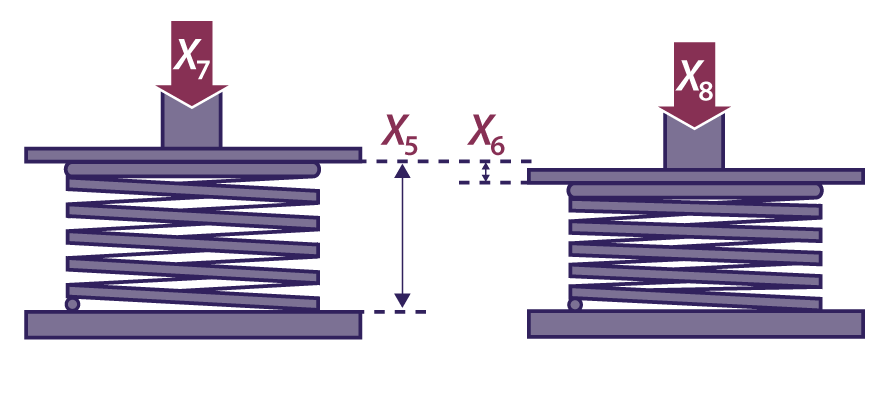
The method of specifying and testing the spring is shown below:
The spring force requirement is 22 +/- 2 Newtons.
The spring force equation, or the Y = f(X) transfer function, is calculated as follows:
Spring Length, L = -X1 + X2 - X3 + X4
Spring Rate, R = (X8 - X7)/X6
Spring Force, Y = X7 + R * (X5 - L)
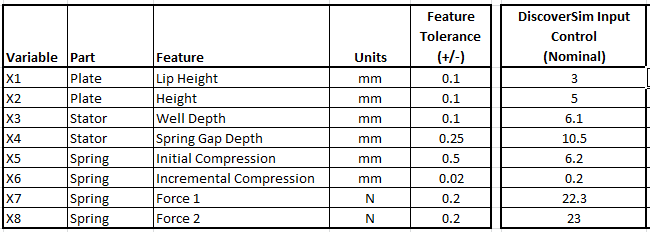
The shut off valve features, tolerances and nominal settings are given as:
In this study we will use DiscoverSim to help us answer the following questions:
What is the predicted process capability with these feature tolerances and nominal
settings?
What are the key X variables that influence spring force Y? Can we improve the process
capability by tightening the tolerance of the important variables? Can this be done
economically?
Can we adjust the nominal settings of X to reduce the transmitted variation in Y,
thereby making the Spring Force robust to the variation due to feature tolerances?
Summary of DiscoverSim Features Demonstrated in Case Study
5:
Create Input Distributions (Continuous Uniform)
DiscoverSim Copy/Paste Cell
Run Simulation with Sensitivity Chart of Correlation Coefficients
Create Continuous Input Controls
Specify Constraints
Run Optimization
Spring Force Simulation and Optimization with DiscoverSim
Open the workbook Shutoff Valve Spring Force.
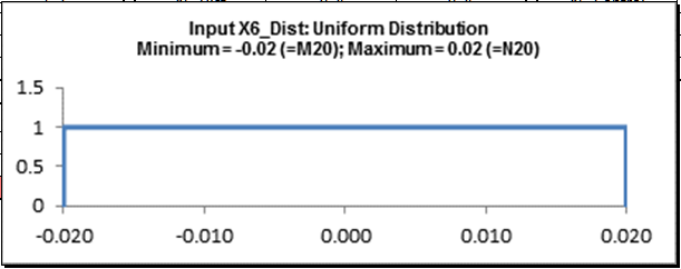
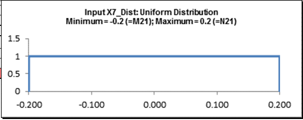
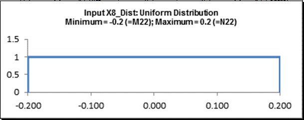
DiscoverSim Input Distributions will simulate the variability in feature tolerance.
We will use the Uniform Distribution, since we do not have historical data to estimate a
best fit distribution, and will assume an equal probability for a feature to have a
minimum tolerance or maximum tolerance value.
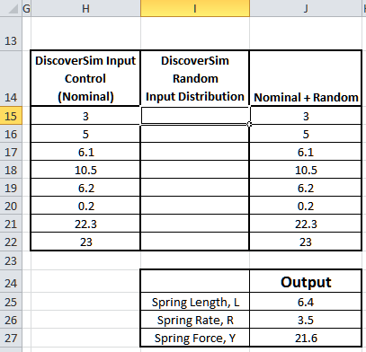
Input Distributions with Uniform Distributions (Random) will be specified in cells
I15 to I22.
Nominal (midpoint) values are specified in cells H15 to
H22 with initial values determined by engineering best estimate.
Input Controls will be applied here for optimization.
The sum of Nominal + Random are used to calculate the X1 to X8 variables and given in
cells J15 to J22.
The output, Spring Rate, will be specified at cell J27 using the
formula given in the introduction.
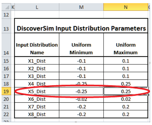
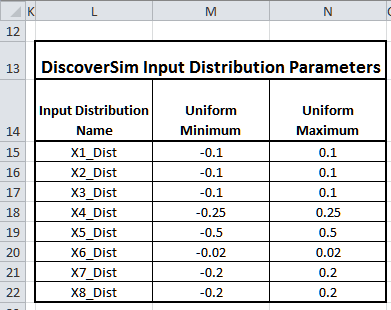
The Input Distribution parameters are given in the following table:
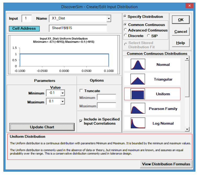
Click on cell I15 to specify the Input Distribution for X1, Lip Height.
Select DiscoverSim > Input Distribution:
Select Uniform Distribution.
Click input Name cell reference and specify cell L15
containing the input name X1_Dist. After specifying a cell reference, the dropdown
symbol changes from to .
Click the Minimum parameter cell reference and specify cell M15 containing the
minimum parameter value = -0.1.
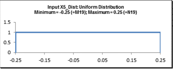
Click the Maximum parameter cell reference and specify cell N15 containing the
maximum parameter value = 0.1.
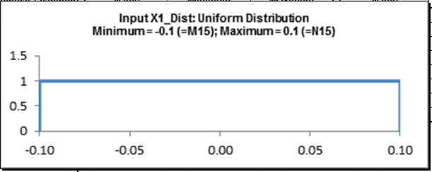
Click Update Chart to view the Uniform Distribution as
shown:
Click OK. Hover the cursor on cell I15 to view the
DiscoverSim graphical comment showing the distribution and parameter values:
Click on cell I15.
Click the DiscoverSim Copy Cell menu button (Do not use Excels Copy it will not
work!).
Select cells I16:I22.
Click the DiscoverSim Paste Cell menu button (Do not use Excels Paste it will not
work!).
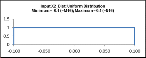
Review the input comments in cells I16 to I22:
Cell I16
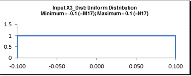
Cell I17
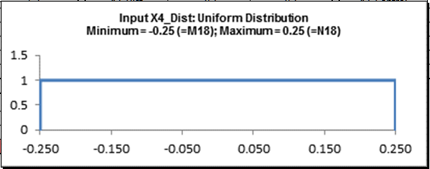
Cell I18
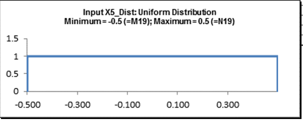
Cell I19
Cell I20
Cell I21
Cell I22
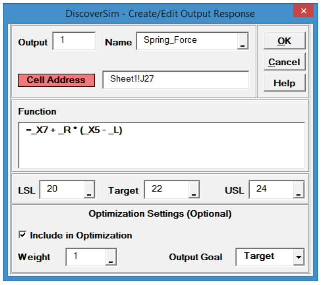
Click on cell J27.
Note: The cell contains the Excel formula for Spring Force:
=_X7 + _R * (_X5 - _L). Excel range names _X7, _R, _X5 and _L are used
rather than cell addresses to simplify interpretation.
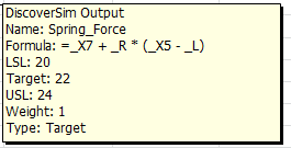
Select DiscoverSim > Output Response:
Enter the output Name as Spring_Force.
Enter the Lower Specification Limit (LSL) as 20,
Target as 22, and Upper Specification Limit (USL) as
24.
Click OK.
Hover the cursor on cell J27 to view the DiscoverSim Output
information.
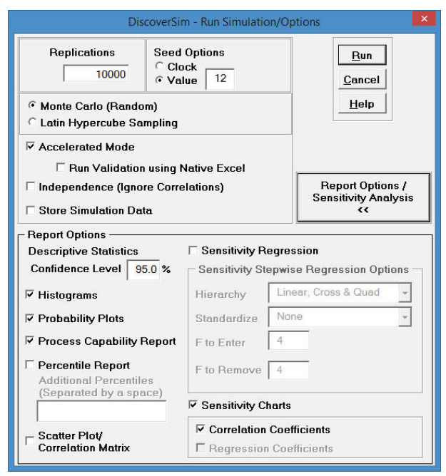
Select DiscoverSim > Run Simulation
Click Report Options/Sensitivity Analysis.
Check Sensitivity Charts and Correlation Coefficients.
Select Seed Value and enter 12 as shown, in order to replicate the
simulation results given below:
Click Run.
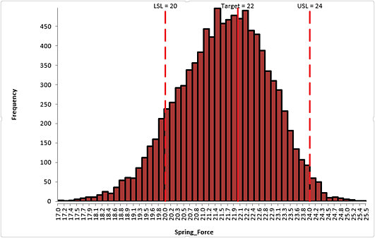
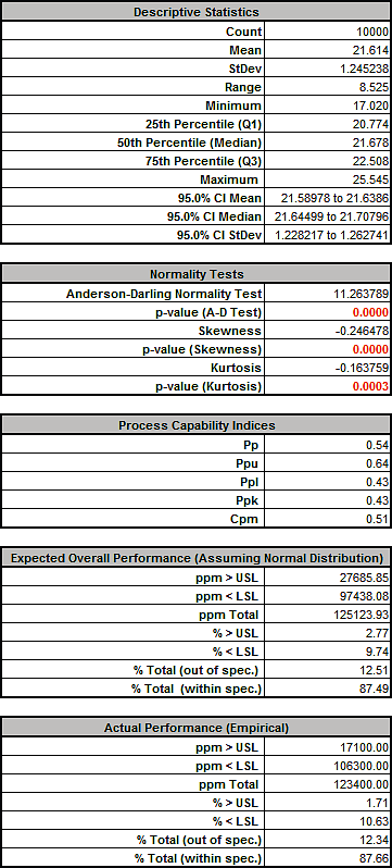
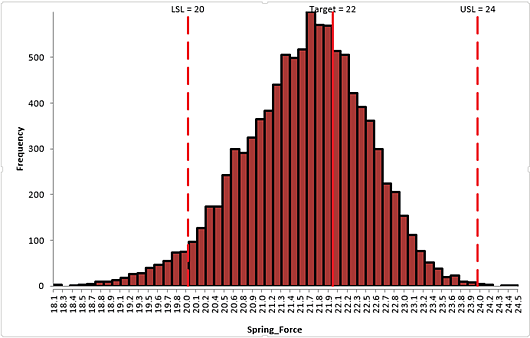
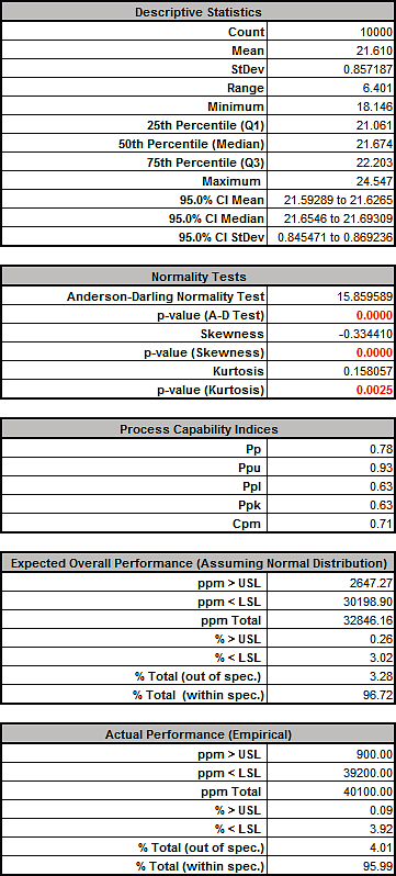
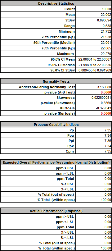
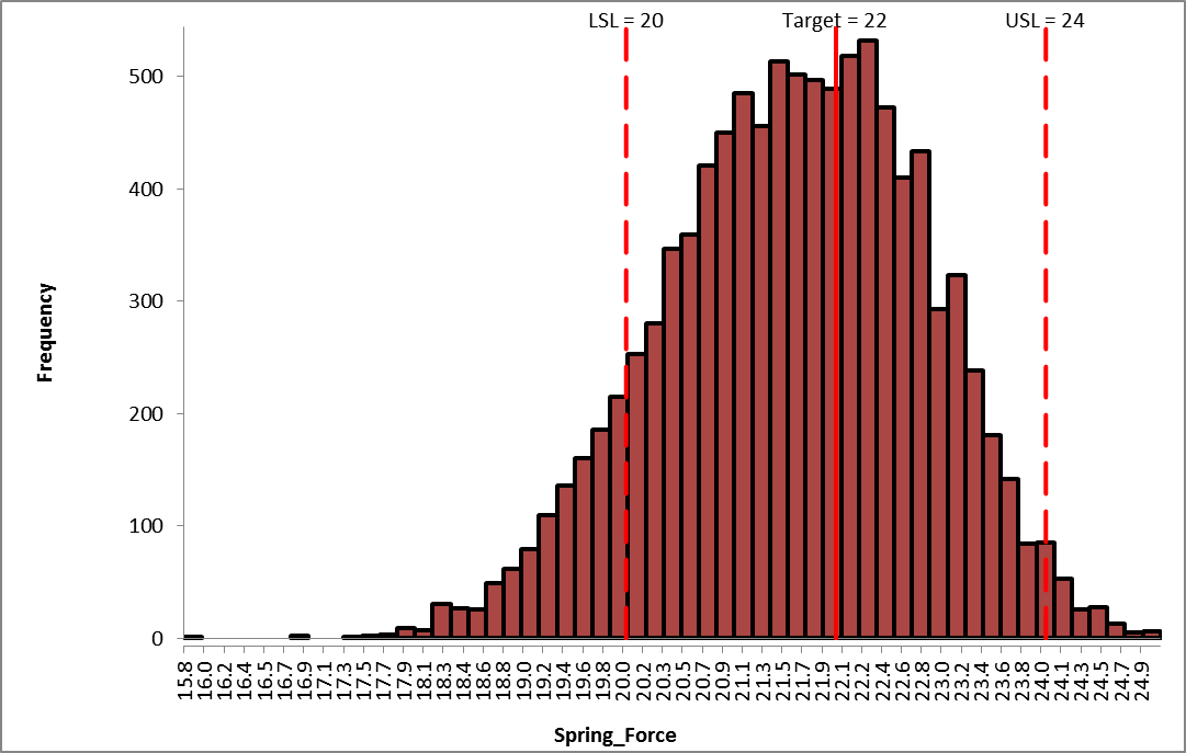
The DiscoverSim Output Report shows a histogram, descriptive statistics and process
capability indices:
From the histogram and capability report we see that the Spring Force is not capable of
meeting the specification requirements.
The process mean is off target and the variation due to feature tolerance is
unacceptably large.
Approximately 12.3% of the shutoff valves would fail, so we must improve this design to
center the mean and reduce the variation.
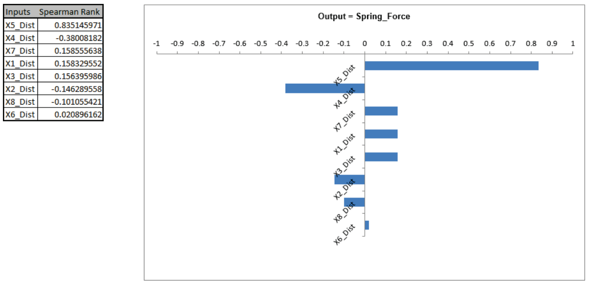
Click on the Sensitivity Correlations sheet:
X5 (Initial Compression) is the dominant input factor affecting Spring Force, followed
by X4 (Spring Gap Depth).
The tolerance on Initial Compression is +/- 0.5.
Discussing this with our supplier it turns out that the tolerance for this spring
feature can be tightened to +/- 0.25 without increasing the cost.
This Sensitivity Chart uses the Spearman Rank Correlation, and the results may be
positive or negative.
If you wish to view R-Squared percent contribution to variation, rerun the simulation
with Sensitivity Regression Analysis and Sensitivity
Charts, Regression Coefficients checked.
Select Sheet1, click on cell M19.
Change the Uniform Minimum value from -0.5 to -0.25.
Click on cell N19. Change the Uniform Maximum value
from 0.5 to 0.25.
DiscoverSim references to cells are dynamic, so this change will take effect on the next
simulation run, but the input comment will need to be refreshed manually.
Click on cell I19 (Input X5_Dist).
Select Input Distribution. Click OK. Review the
revised input comment in cell I19:
Rerun the simulation without sensitivity charts:
Tightening the tolerance of X5, Initial Compression resulted in an improvement with the
Spring Force standard deviation reduced from 1.24 to 0.86, actual percent out of
specification from 12.5 to 4.0% and Ppk increased from .43 to .63.
However a Six Sigma design should have a minimum Ppk value of 1.5.
At this point one could use Excels Solver to further improve the process by finding the
nominal values that center the mean, but that still would not achieve the desired
quality level.
DiscoverSims Stochastic Global Optimization will not only find the optimum X settings
that result in the best mean spring force value, it will also look for a solution that
will reduce the standard deviation.
Stochastic optimization looks for a minimum or maximum that is robust to variation in X,
thus reducing the transmitted variation in Y.
This is referred to as Robust Parameter Design in Design For Six Sigma (DFSS).
In order to run optimization, we will need to add Input Controls (also known as Decision
Variables).
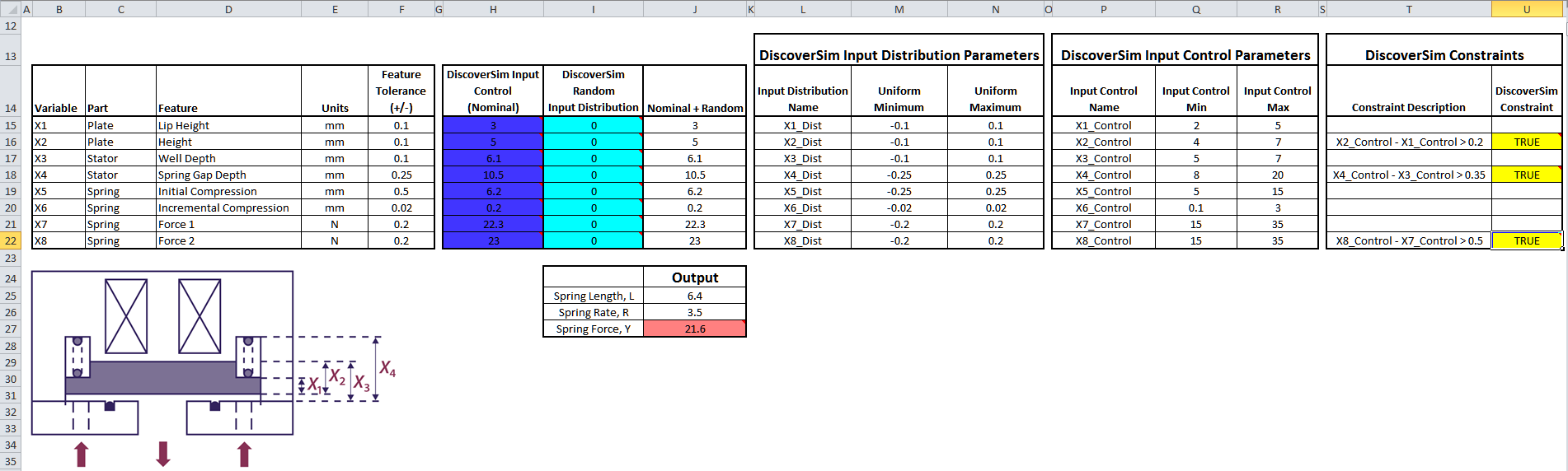
Select Sheet1.
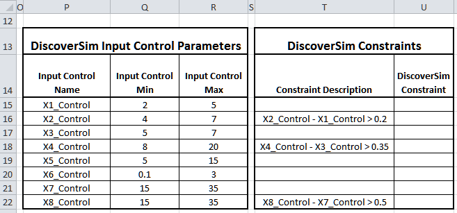
The Input Control parameters are given in the table:
The controls will vary the nominal X values in H15 to
H22.
The nominal values are added to the random input distribution (J15 to
J22) as discussed above in Step 1.
Constraints will also be added as shown so that there can be no overlap due to
tolerance.
For example if X2, Height, was at the low end of its tolerance and X1, Lip Height, was
at the high end of its tolerance, it is possible that an overlap would leave no place
for the spring to be seated.
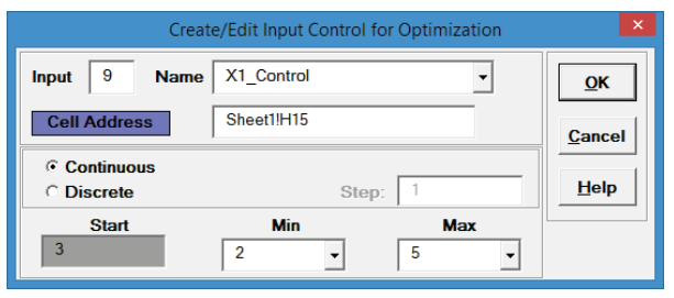
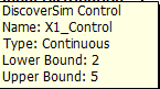
Click on cell H15. Select Control:
Click input Name cell reference and
specify cell P15 containing the input control name X1_Control.
Click the Min value cell reference and
specify cell
Q15 containing the minimum optimization boundary value = 2.
Click the Max value cell reference and
specify cell R15 containing the maximum optimization boundary value =
5:
Click OK. Hover the cursor on cell H15 to view the
comment displaying the input control settings:
Click on cell H15.
Click the DiscoverSim Copy Cell menu button (Do not use Excels Copy it will not
work!).
Select cells H16:H22.
Click the DiscoverSim Paste Cell menu button (Do not use Excels Paste it will not
work!).
Review the input control comments in cells H16 to H22.
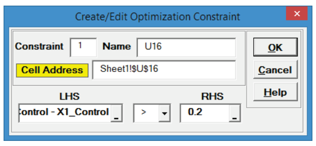
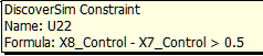
Now we will add the Constraints. Click on cell U16.
Select Constraint:
Type X2_Control X1_Control in the Left Hand Side
(LHS).
Select Greater Than >.
Enter 0.2 in the Right Hand Side (RHS).
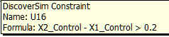
Click OK. Review the comment at cell U16.
The cell display is TRUE since the initial value for X2_Control (5) is greater than
the initial value for X1_Control (3).
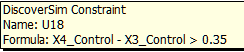
Repeat steps 33 and 35 with constraints at cells U18 and
U22 as shown:
The completed model is shown below:
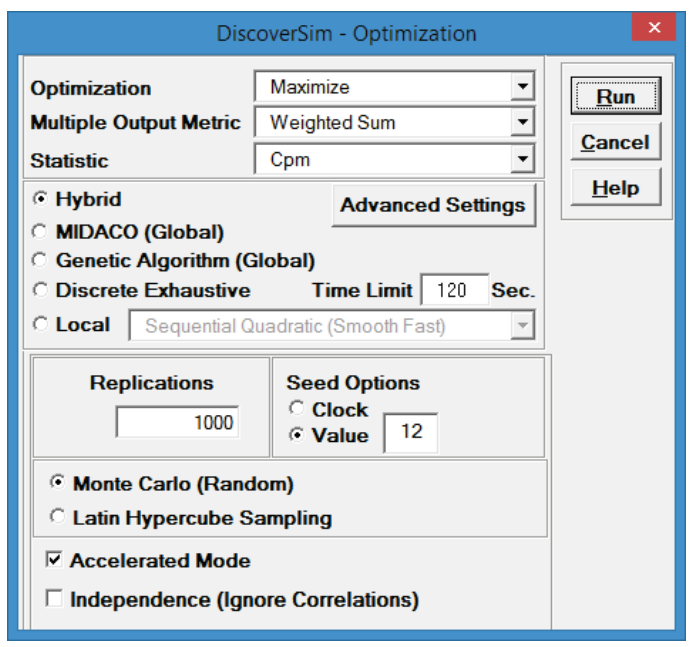
Now we are ready to perform the optimization. Select DiscoverSim >
Run Optimization:
Select Maximize for Optimization Goal, Weighted Sum for
Multiple Output Metric and Cpm for Statistic.
Select Seed Value and enter 12, in order to replicate the
optimization results given below.
Set Replications to 1000 to reduce the optimization time. All other
settings will be default as shown:
Maximize Cpm is used here, rather than Ppk, because it incorporates a penalty for mean
deviation from target. We want the spring force mean to be on target with minimal
variation.
Note, however, that this solution may not produce the lowest possible standard
deviation.
We will use the Hybrid optimization method which requires more time to
compute, but is powerful to solve complex optimization problems.
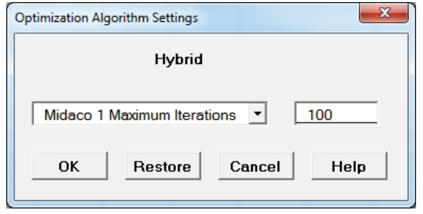
Tip: To speed up this optimization, change the maximum number of
iterations in Hybrid Midaco 1 (first MIDACO run) from 1000 to 100.
Click Advanced Settings.
Select Midaco 1Maximum Iterations. Enter 100 as shown.
Click OK.
Click Run.
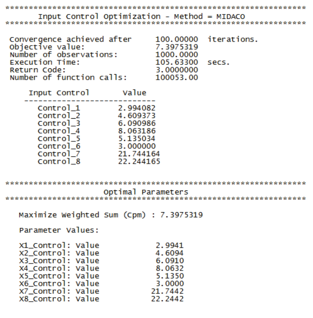
Scroll through the optimization report window to view the various optimization methods.
The initial method in Hybrid, DIRECT global optimization, found a solution that resulted
in a very good Cpm value of
7.4:
The Genetic Algorithm uses the above optimal values as a starting point, but is unable
to further improve on MIDACOs Cpm value of 7.4.
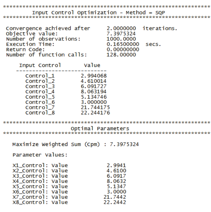
The final method in this Hybrid, Sequential Quadratic Programming local optimization,
uses the Genetic Algorithm optimal values as a starting point but is unable to further
improve on the Cpm value of 7.4.
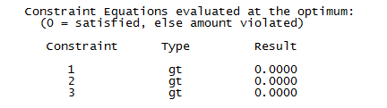
The constraint equations evaluated at this optimum are satisfied:
Note: The constraint cell values in Excel will all appear as TRUE at
the optimum.
You are prompted to paste the optimal values into the spreadsheet:
Click Yes.
This replaces the nominal input control values to the optimum values.
Select Run Simulation. Click Run.
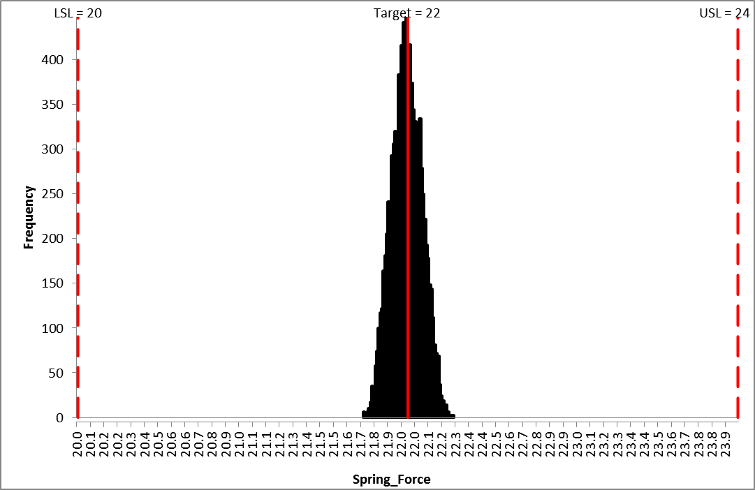
The resulting simulation report confirms the predicted dramatic improvement:
The slight discrepancy in predicted Cpm (Optimization 7.4 versus Simulation 7.35 is due
to the difference in number of replications for Optimization (1000) versus Simulation
(10,000).
Recall the histogram for the initial simulation run:
In summary, DiscoverSim was used to dramatically improve the Spring Force performance as
follows:
Mean centered from 21.6 to 22.0
Standard Deviation reduced from 1.24 to 0.09, more than a ten-fold reduction!
Ppk increased from 0.43 to 7.23, Cpm increased from 0.51 to 7.35!
Actual % Total (out of spec) reduced from 12.3% to 0%!
The benefits do not stop here. Since the design is now so robust, we can review the
input tolerances to see if there is a cost saving opportunity by widening the feature
tolerances, and re-running the simulation to study the impact.
Finally the results predicted here should be validated with physical prototypes before
proceeding to finalize the design parameters. Remember All models are wrong, some are
useful! George Box.

 to
to  .
.
 (Do not use Excels Copy it will not
work!).
(Do not use Excels Copy it will not
work!).
 (Do not use Excels Paste it will not
work!).
(Do not use Excels Paste it will not
work!).