Case Study 3 Six Sigma DMAIC Project Portfolio Selection
Introduction: Optimizing DMAIC Project Portfolio to Maximize Cost Savings
This is an example of DiscoverSim optimization used to select Six Sigma DMAIC projects that
maximize expected cost savings.
This example model was contributed by: Dr. Harry Shah, Business Excellence Consulting.
The goal is to select projects that maximize Total Expected Savings subject to a constraint
of Total Resources <= 20. Management requires a minimum total project savings of $1 Million
(Lower Specification Limit, LSL=1000 $K). We will explore the optimal selection of
projects that maximize the Mean Savings and also consider maximizing the Process
Capability Index Ppl.
Cost Savings are specified with a Triangular Distribution.
The Probability of Success is modeled using the Bernoulli (Yes/No) Distribution.
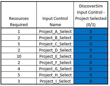
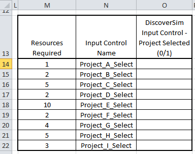
Resources Required are specified for each project. DiscoverSim Input Controls
(Discrete) are used to select the project (0,1).
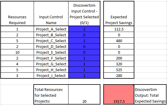
Expected Project Savings are calculated as the sum of: Cost Savings * Probability of
Success (if project is selected) or 0 (if project is not selected).
Summary of DiscoverSim Features Demonstrated in Case
Study 3:
Optimization of Project Portfolio with DiscoverSim
Open the workbook DMAIC Project Selection - Optimization.
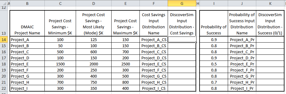
DiscoverSim Input Distributions will simulate the variability in the cost
savings and probability of success for each project. We will specify cost
savings as a Triangular Distribution for each project in cells
G14 to G22. The probability of success will be
specified at cells
K14 to K22 using the Bernoulli (Yes/No)
Distribution.
DiscoverSim Input Controls (Discrete) will be used to select the project (0,1)
and specified in cells
O14 to O22.
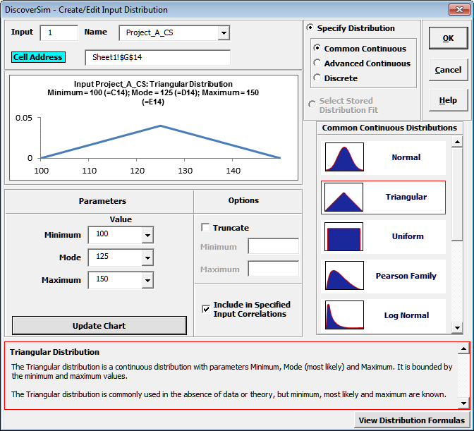
Click on cell G14 to specify the Cost Savings Input
Distribution for Project_A. Select
DiscoverSim > Input Distribution:
Select Triangular Distribution.
Click the input name cell reference and specify
cell
F14 containing the input Name Project_A_CS
(denoting Project A Cost Savings). After specifying a cell reference, the
dropdown symbol changes from to .
Click the Minimum parameter cell reference and specify cell
C14 containing the minimum parameter value = 100 ($K).
Click the Mode parameter cell reference and specify cell
D14 containing the mode (most likely) parameter value = 125
($K).
Click the Maximum parameter cell reference and specify cell
E14 containing the maximum parameter value = 150 ($K).
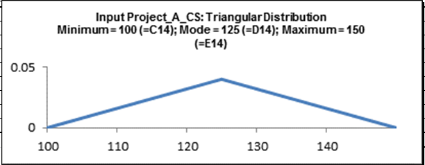
Click Update Chart to view the Triangular
Distribution as shown:
Click OK. Hover the cursor on cell G14 to view
the DiscoverSim graphical comment showing the distribution and parameter values:
Click on cell G14. Click the DiscoverSim Copy
Cell menu button
(Do not use Excels Copy it will not work!).
Select cells G15:G22. Now click the DiscoverSim Paste
Cell menu button (
Do not use Excels Paste it will not work!).
Review the input comments in cells G15 to G22.
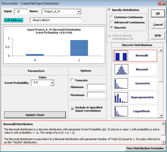
Click on cell K14 to specify the Probability of Success Input
Distribution for Project_A. Select
DiscoverSim > Input Distribution:
Select Discrete and Bernoulli Distribution.
Bernoulli is also sometimes referred to as the Yes/No distribution.
Click the input Name cell reference and specify cell
J14 containing the input name Project_A_Pr (denoting Project
A Probability of Success).
Click the Event Probability parameter cell reference and
specify cell I14 containing the probability parameter value =
0.9.
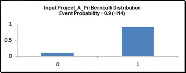
Click Update Chart to view the Bernoulli distribution as shown:
Click OK. Hover the cursor on cell K14 to view
the DiscoverSim graphical comment showing the distribution and parameter values:
Click on cell K14. Click the DiscoverSim Copy
Cell menu button (Do not
use Excels Copy it will not work!).
Select cells K15:K22. Now click the DiscoverSim Paste
Cell menu button (Do not
use Excels Paste it will not work!).
Review the input comments in cells K15 to K22.
Now we will add Discrete Input Controls (also referred to as Decision
Variables). These will be used to select the project (0 denotes project not
selected, 1 denotes project selected). DiscoverSim will use stochastic global
optimization to determine which projects to select and which not to select in
order to maximize total cost savings. A constraint will also be added to ensure
that the total number of resources is
<=2 0.
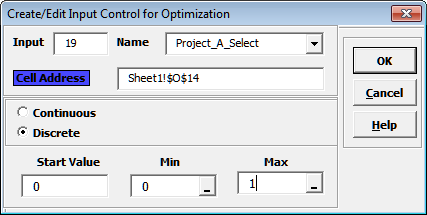
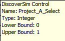
Click on cell O14. Select Control:
Click input Name cell reference
and specify cell N14 containing the input control name
Project_A_Select.
Select Discrete (this input control setting will consider only
integer values). Set the
Max value to 1 as shown:
Click OK. Hover the cursor on cell O14
to view the comment displaying the Input Control settings:
Click on cell O14. Click the DiscoverSim Copy
Cell menu button (Do not
use Excels Copy it will not work!).
Select cells O15:O22. Click the DiscoverSim Paste
Cell menu button (Do not
use Excels Paste it will not work!).
Review the input control comments in cells O15 to
O22.
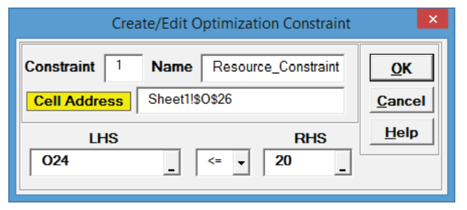
Now we will add the constraint. Click on cell O26. Select
Constraint:
Enter the Constraint Name as Resource_Constraint. Enter
O24 in the Left Hand Side (LHS) or
click the LHS cell reference
and select O24. Select
<=. Enter 20 in the Right Hand Side (RHS).
Note: Cell O24 contains
the Excel formula: =SUMPRODUCT(O14:O22,M14:M22). This sums the product of
resources*selected(0,1), in other words the sum of selected project resources.
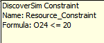
Click OK. Review the comment at cell O26.
The cell display is TRUE since the initial value for
O24 is zero which obviously satisfies the constraint.
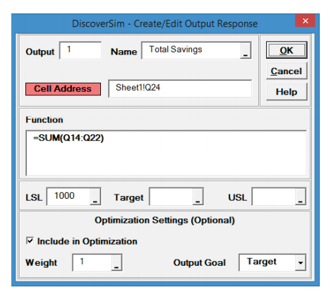
Now we will specify the output. Click on cell Q24. The cell
contains the Excel formula for the sum of expected savings as the sum of: Cost
Savings * Probability of Success (if project is selected) or 0 (if project is
not selected).
Select DiscoverSim > Output Response:
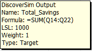
Enter the output Name as Total_Savings. Enter the Lower
Specification Limit (LSL) as 1000.
The Weight and Output Goal settings are used
only for multiple response optimization, so do not need to be modified in this
example.
Click OK.
Hover the cursor on cell Q24 to view the DiscoverSim Output
information.
Now we are ready to perform the optimization to select projects. Select
DiscoverSim > Run Optimization:
Select Maximize for Optimization Goal and Mean for
Statistic. Select Seed Value and enter 12 in
order to replicate the optimization results given below. Change
Replications to 1000 to reduce the optimization time. All other
settings will be default as shown:
Note: Maximize Mean may not produce the lowest possible
standard deviation, so we will consider Maximize Ppl later.
We will use the Hybrid optimization method which requires more
time to compute, but is very powerful to solve complex optimization problems.
Since this is a small discrete problem,
Discrete Exhaustive will be used. If there were more projects, say 20, then
MIDACO would have been used.
Click Run.
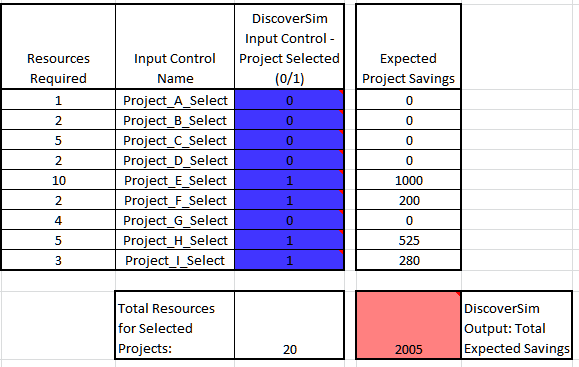
The final optimal parameter values are given as:
Projects E, F, H and I have been selected giving a predicted mean cost savings
of 2004 ($K). Intuitively, these would be the projects one would select given
that they have the highest expected values per resource. However, a simple pick
the winner approach fails to take into account the variability and likelihood
of meeting the minimum total cost saving requirement of 1000 $K.
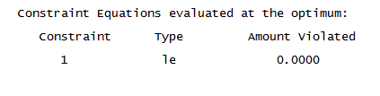
The constraint equation evaluated at this optimum has been satisfied (amount
violated = 0):
Project E requires 10 resources, F requires 2, H requires 5 and I requires 3 for
a total of 20, satisfying our constraint that the total resources be less than
or equal to 20.
You are prompted to paste the optimal values into the spreadsheet:
Click Yes. This sets the Input Control values to the optimum
values as shown:
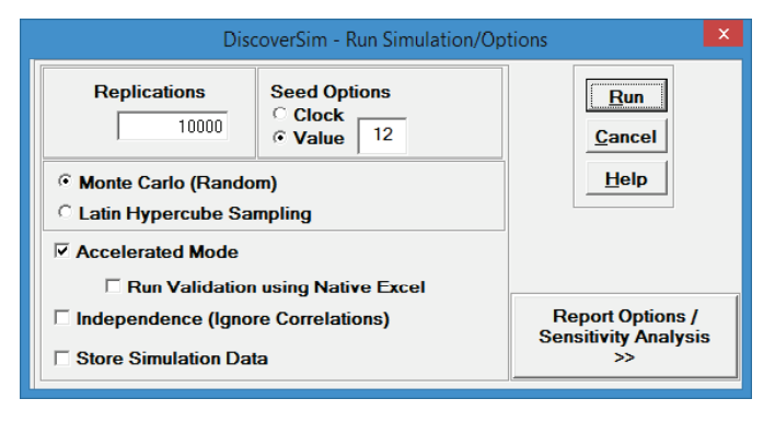
Select DiscoverSim > Run Simulation:
Select Seed Value and enter 12 as shown, in order to
replicate the simulation results given below.
Click Run.
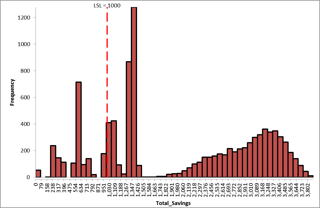
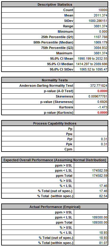
The DiscoverSim Output Report displays a histogram, descriptive statistics and
process capability indices:
From the histogram and capability report we see that the expected mean total
savings are good (2011 $K), but the standard deviation is very large (1080 $K).
Looking at the Actual Performance report we see that there is an 18.9% chance of
failing to meet the management requirement of 1000 $K.
Now we will rerun the optimization to select projects, but this time, we will
maximize the process capability index Ppl.
(Ppl is used since we only have a lower specification limit).
This will simultaneously maximize the mean and minimize the standard
deviation:
Ppl = (Mean
LSL)/(3*StDev).
An equivalent alternative would be to minimize Calculated DPM.
Note: A nonparametric alternative statistic would be %Ppl
(percentile Ppl):
%Ppl = (Median
LSL)/(Median - 0.135 Percentile).
This is robust to the assumption of normality. Another robust statistic would be
Actual DPM.
With either of these we would recommend increasing the number of replications to
10,000 to improve the precision of the statistic, but this would require
significantly more computation time for optimization.
Reset the project selection by changing the Input Control values to 0:
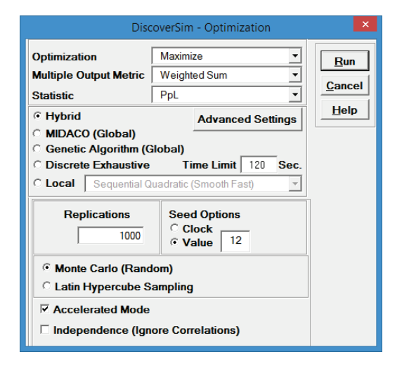
Select DiscoverSim > Run Optimization
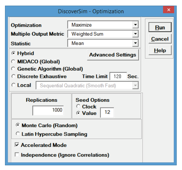
Select Maximize for Optimization Goal, Weighted Sum for
Multiple Output Metric and PpL for
Statistic. Select
Seed Value and enter 12, in order to replicate the
optimization results given below. Set
Replications to 1000 to reduce the optimization time. All other
settings will be default as shown:
Click Run.
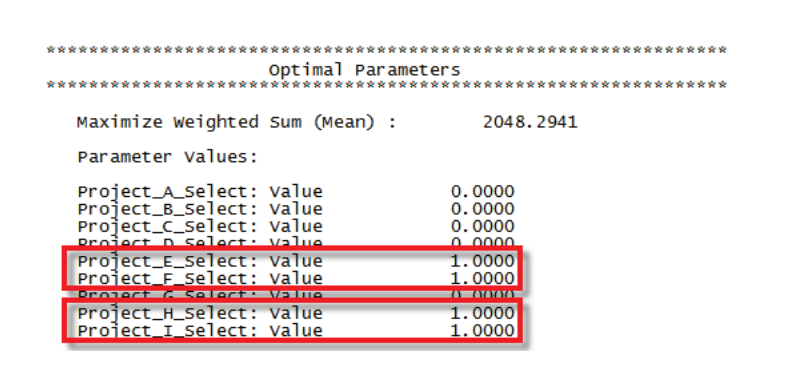
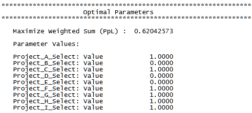
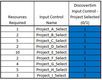
The final optimal parameter values are given as:
Projects A, C, F, G, H, and I have been selected giving a predicted Ppl of
0.62.
Note: Project E, previously selected to maximize the mean, was
not selected when the goal was to maximize the process capability, Ppl.
The constraint requirement that the total number of resources be
<=2 0 is satisfied with this selection.
You are prompted to paste the optimal values into the spreadsheet:
Click Yes.
This sets the Input Control values to the optimum values as shown:
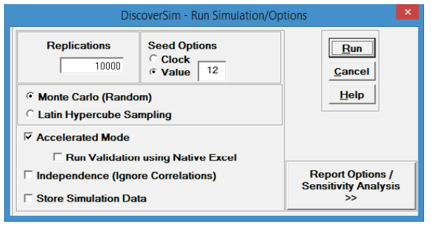
Select DiscoverSim > Run Simulation:
Select Seed Value and enter 12 as shown, in order to
replicate the simulation results given below.
Click Run.
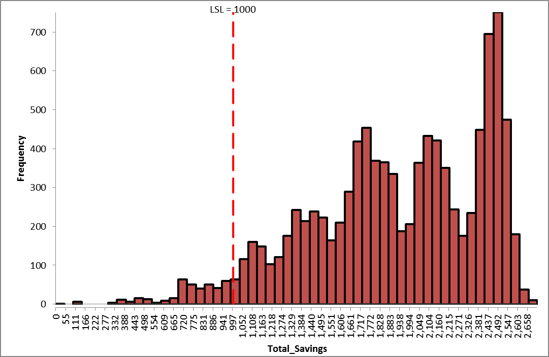
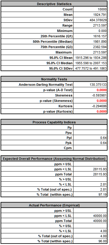
The DiscoverSim Output Report displays a histogram, descriptive statistics and
process capability indices:
Note that the mean total savings have been reduced somewhat from 2011 to 1925
$K, however, the standard deviation has been reduced from 1080 to 484 $K and the
chance of failing to meet the management requirement of 1000 $K has been reduced
from 18.9% to 4.0% (actual performance).
Considering the two selection scenarios, one can present the risks to management
and make the project selection decision to go either way: take the risk and
maximize the mean with potential larger savings, or choose the safer projects
that result in less variation and significantly improve the chance of meeting a
minimum savings of 1 million.
Clearly, Project E is the key project to consider in this analysis. The impact
of this project can be confirmed with a sensitivity analysis.
Set all of the Input Control values to 1 as shown:
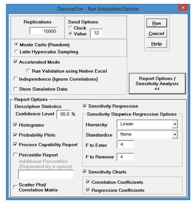
Select DiscoverSim > Run Simulation:
Click Report Options/Sensitivity Analysis. Check
Sensitivity Regression Analysis, Sensitivity Charts -
Correlation Coefficients and
Regression Coefficients. Select Seed Value and
enter 12 as shown, in order to replicate the simulation results given below.
Click Run.
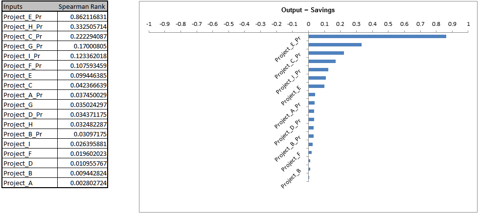
Click on the Sensitivity Correlations sheet:
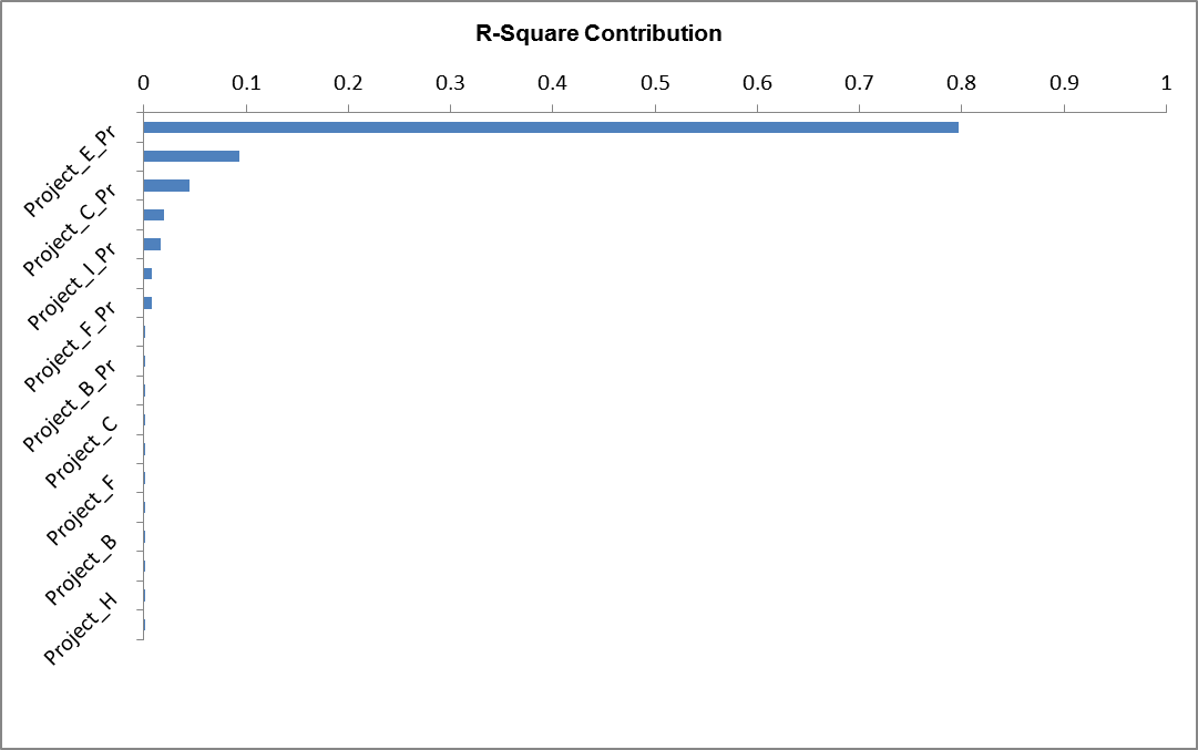
Click on the Sensitivity Regression sheet to view the R-Square
percent contribution to variation:
The sensitivity charts confirm that Project E is the dominant X factor. This
is a high impact project, but is also a difficult project with a probability of
success of only 0.5 and a large variation (min = 2000, max = 2500). If possible,
this project might be split into smaller, lower risk (higher probability of
success) projects with less variation.
Optional Insert DSIM Function: As an alternative to Maximize
CpL as shown above, we could also Maximize Mean Savings subject to an added
constraint that the Standard Deviation of Savings be < 500. Click on cell
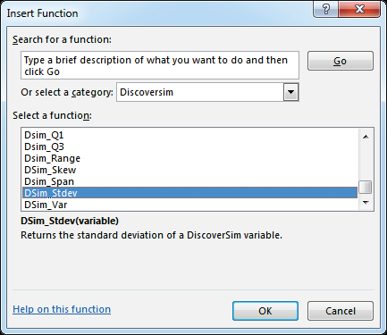
Q27 and select DiscoverSim > DSIM
Function:
Scroll down to select DSIM_Stdev. Click OK.
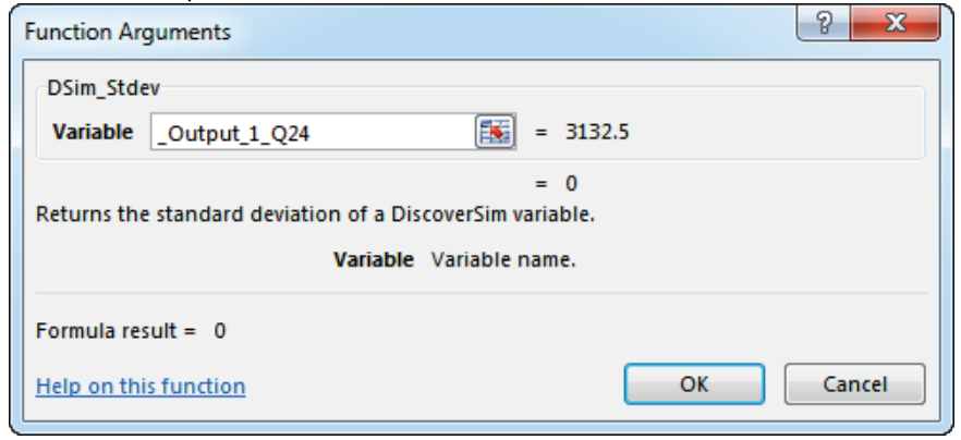
Select the Output Q24 as the DSIM Variable.
The DiscoverSim Range Name for Q24
is _Output_1_Q24. Click OK.
The DSIM function formula is now in cell = DSim_Stdev(_Output_1_Q24)
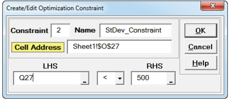
Now we will add a constraint at cell O27 that references the
DSIM function. Click on cell O27. Select
Constraint:
Enter the Constraint Name as StDev_Constraint. Enter
Q27 in the Left Hand Side (LHS) or click the
LHS cell
reference and
select Q27. Select <. Enter 500 in the
Right Hand Side (RHS).
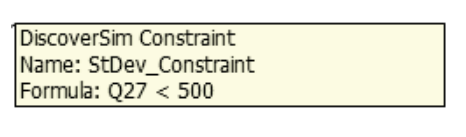
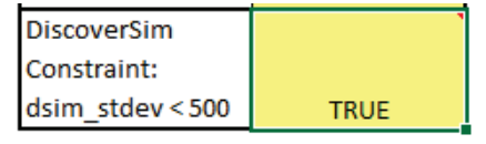
Click OK. Review the comment at cell O27:
The cell display is TRUE since the initial value for Q27 is
zero which obviously satisfies the constraint.
With all of the Input Control values set to 1, select DiscoverSim >
Run Optimization:
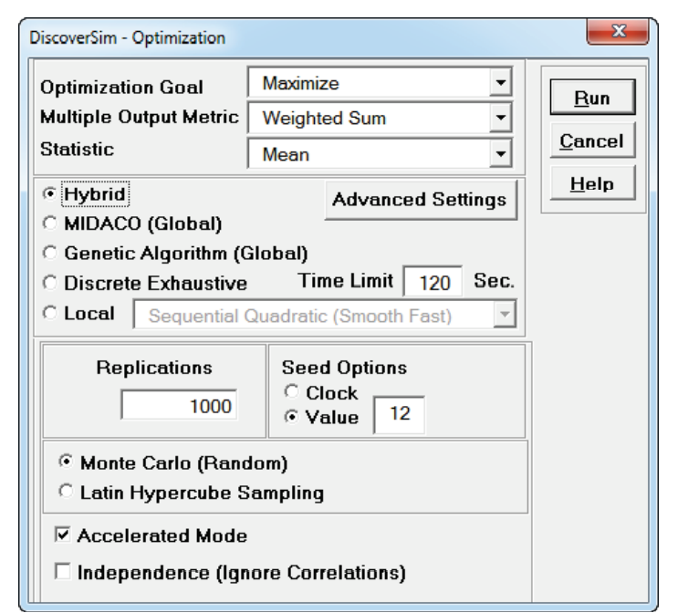
Select Maximize for Optimization Goal, Weighted Sum for
Multiple Output Metric and Mean for
Statistic.
Select Seed Value and enter 12, in order to replicate the
optimization results given below.
Set Replications to 1000 to reduce the optimization time.
All other settings will be the defaults as shown:
Click Run.
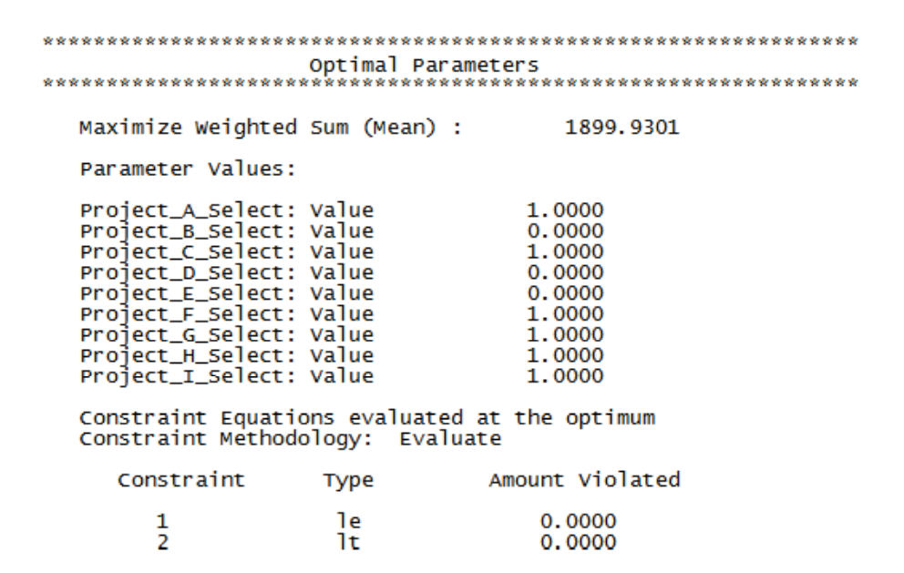
The final optimal parameter values are given as:
Projects A, C, F, G, H, and I have been selected giving a predicted Mean of
1899.9. These are exactly the same projects that were selected above with
maximize PpL.
You are prompted to paste the optimal values into the spreadsheet:
Since we have already analyzed this project selection, we will not pursue this
further. Click No.
The use of Insert DSIM Function as shown provides flexibility
in specifying the optimization objective function. For example in a multiple
output scenario, you can Maximize the Mean of Output 1, with a constraint that
Output 2 Ppk process capability must be > 1.


 and specify
cell
F14 containing the input Name Project_A_CS
(denoting Project A Cost Savings). After specifying a cell reference, the
dropdown symbol changes from
and specify
cell
F14 containing the input Name Project_A_CS
(denoting Project A Cost Savings). After specifying a cell reference, the
dropdown symbol changes from  .
.
 (Do not use Excels Copy it will not work!).
 (
Do not use Excels Paste it will not work!).
(
Do not use Excels Paste it will not work!).