This is an example of DiscoverSim Monte Carlo simulation to determine probability of daily
profit using a basic profit model for a small retail business. We will apply distribution
fitting to historical data and specify input correlations to define the model in a way that
closely matches our real world business.
The profit (Pr) requirement is Pr > 0 dollars (i.e., the lower specification limit LSL = 0)
The profit equation, or Y = f(X) transfer function, is calculated as follows:
Total Revenue, TR = Quantity Sold * Price
Total Cost, TC = Quantity Sold * Variable Cost + Fixed Cost
Profit, Pr = TR TC
In this study we will use DiscoverSim to help us answer the following questions:
What is the predicted probability of daily profit?
What are the key X variables that influence profit Y? Can we reduce the variation in
profit by reducing the variation of the important input variables?
Summary of DiscoverSim Features Demonstrated in
Case Study 1:
Distribution Fitting Discrete Batch Fit
Distribution Fitting Continuous Batch Fit
Distribution Fitting Specified Distribution Fit
Create Input Distributions with Stored Distribution Fit
Specify Input Correlations
Run Simulation and display
Histograms, Descriptive Statistics, Process Capability Report
Percentile Report
Scatter Plot/Correlation Matrix
Sensitivity Chart of Correlation Coefficients
Sensitivity Chart of Regression Coefficients
Distribution Fitting Nonnormal Process Capability
Profit Simulation with DiscoverSim
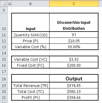
Open the workbook Profit Simulation. DiscoverSim Input Distributions
will simulate the variability in Quantity Sold, Price and Variable Cost. We will use
distribution fitting with historical data to determine which distributions to use and
what parameter values to enter. Input Distributions will then be specified in
cells C11,
C12 and C13. The output, Profit, will be specified at
cell
C21 using the formula given above.
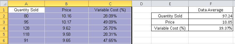
Select the Historical_Data sheet. This gives historical data for
Quantity Sold, Price and Variable Cost.
Tip: At this point use the SigmaXL tool (bundled with DiscoverSim) to
obtain descriptive statistics to test for normality (SigmaXL >
Statistical Tools > Descriptive Statistics).
Quantity Sold has an Anderson Darling Normality test p-value = 0.83, so may be
considered as a Normal Distribution, but since it is a count we will apply DiscoverSims
distribution fitting using discrete distributions.
Price and Variable Cost are non-normal with AD p-values less than .05,
so we will use DiscoverSims distribution fitting for continuous data. SigmaXLs
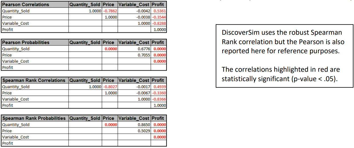
correlation matrix should also be used to evaluate correlations
(SigmaXL >
Statistical Tools > Correlation Matrix). The
Spearman Rank correlation for Quantity Sold versus Price is -0.8 (Note:
DiscoverSim uses the more robust Spearman Rank correlation rather than Pearsons
correlation). SigmaXLs graphical tools such as Histograms and Scatterplots should also
be used to view the historical data.
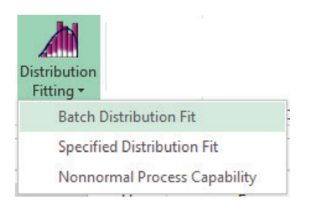
Select DiscoverSim > Distribution Fitting >
Batch Distribution Fit:
The data range has been preselected and appears in the dialog.
Note: if a different range is required, click on to change it or select
Use Entire Data Table to automatically select the data.
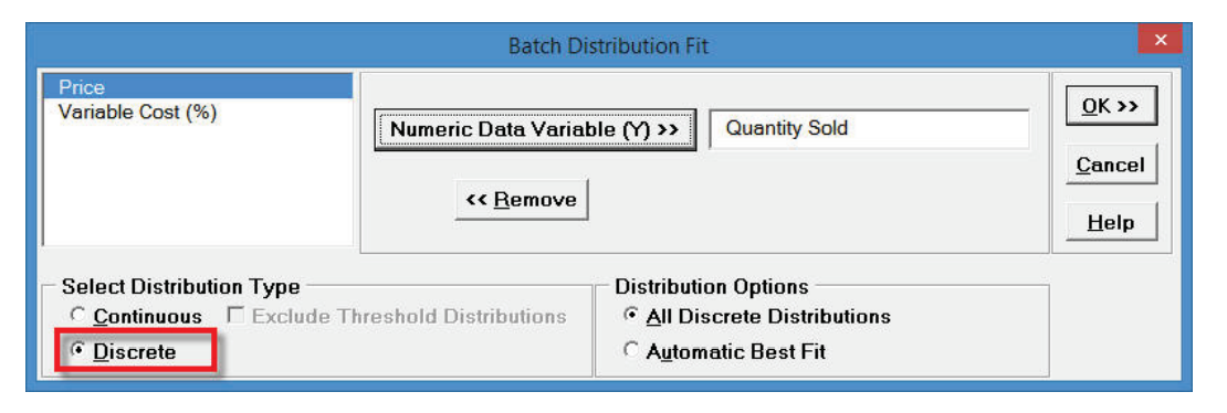
Click Next. Since Quantity Sold is
count data, i.e. a discrete variable, select Discrete. Select
Quantity Sold as the
Numeric Data Variable (Y). For
Distribution Options use the default All Discrete Distributions
as shown:
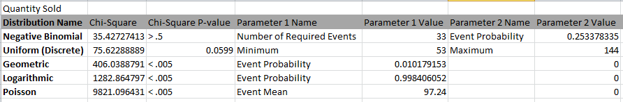
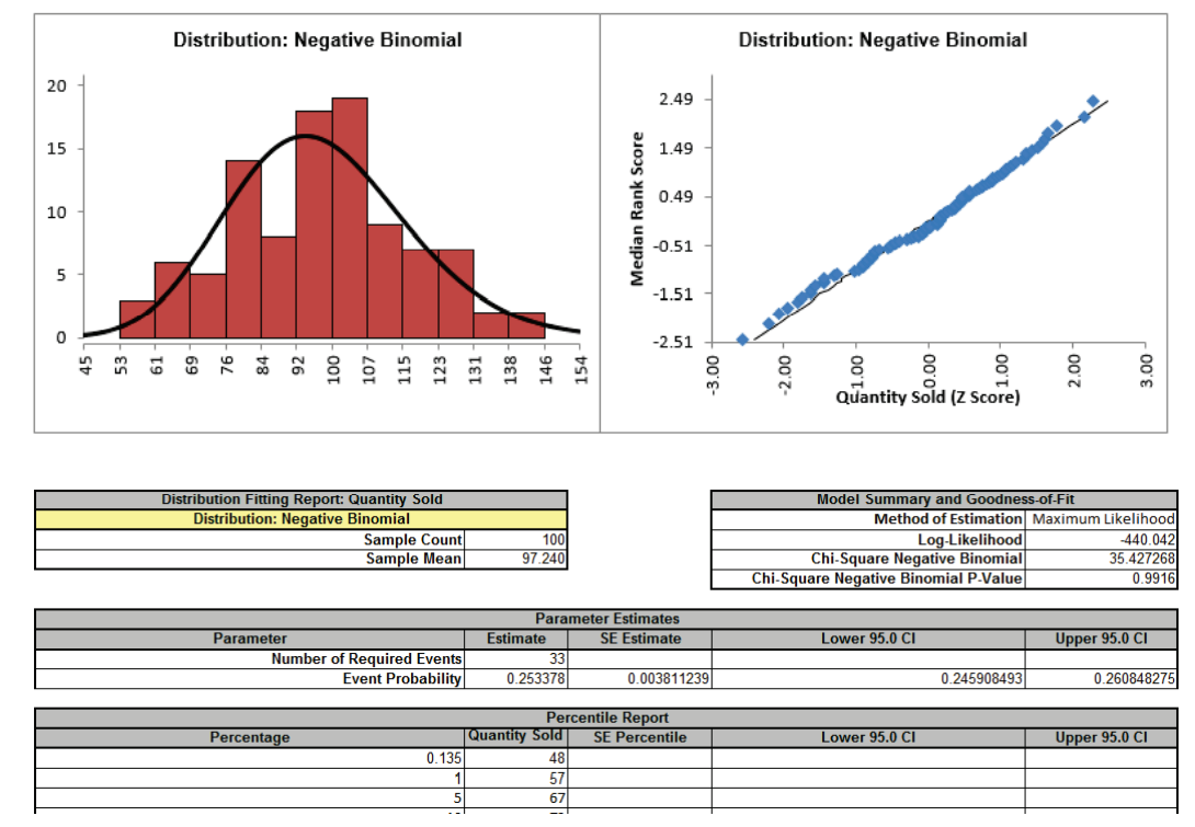
Click OK. The resulting discrete distribution report is shown below:
Since these are discrete distributions, Chi-Square is the statistic used to determine
goodness-of-fit. The distributions are sorted by Chi-Square in ascending order. The
best fit distribution is
Negative Binomial with Chi-Square = 35.4 and p-value =
0.99. The parameters are
Number of Required Events = 33 and Event
Probability
= 0.2534.
Tip: If the best fit discrete distribution has a p-value less
than .05 indicating a poor goodness-of-fit, none of the discrete distributions
are adequate for use in Monte-Carlo simulation. In this case you should redo the
distribution fit using the
Continuous option (Note that you can use the continuous option for
discrete data, but you cannot use discrete distributions for continuous data). After
creating a DiscoverSim input distribution with the best fit (or normal if
applicable), use Excels ROUND(number, 0) function to obtain integer values
from the continuous distribution.
Now we will apply distribution fitting to Price and Variable Cost.
Select the
Historical_Data sheet and repeat the above steps. Both variables are
continuous so use the default
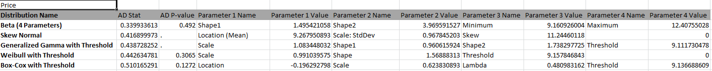
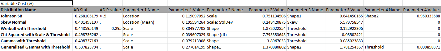
Select Distribution Type Continuous. The resulting distribution reports
are shown below.
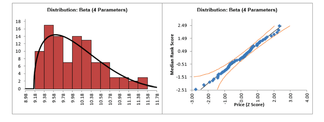
DiscoverSim uses the Anderson Darling statistic to determine goodness-of-fit for
continuous distributions. The distributions are sorted by the AD statistic in ascending
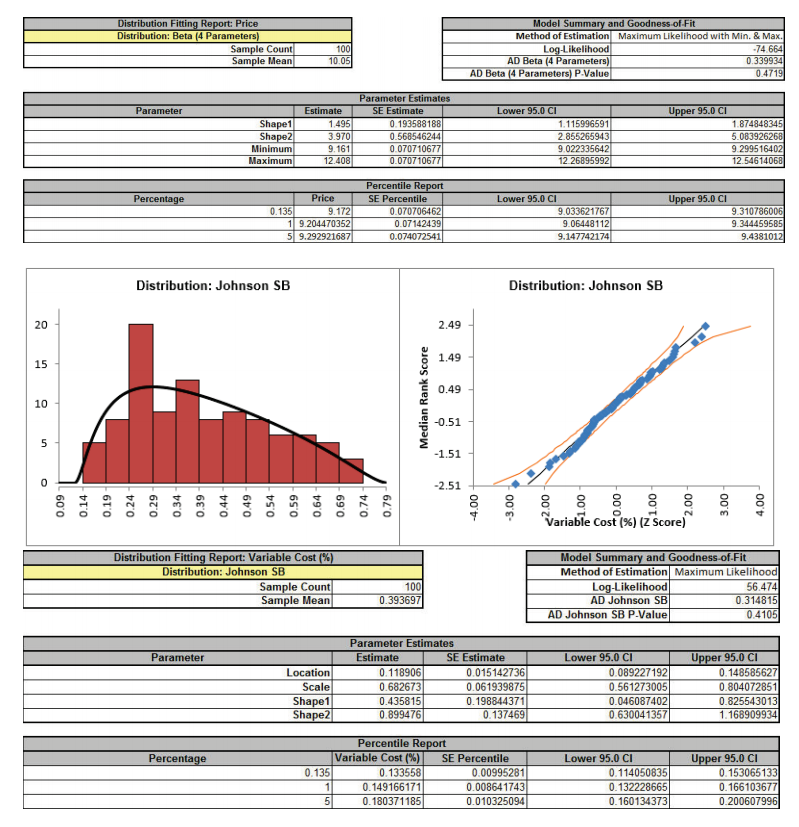
order. The best fit distribution for
Price is
Beta (4 Parameters) with AD Stat = .34 and AD p-value = 0.47. The best
fit distribution for
Variable Cost (%) is
Johnson SB with AD Stat = .31 and AD p-value = 0.41
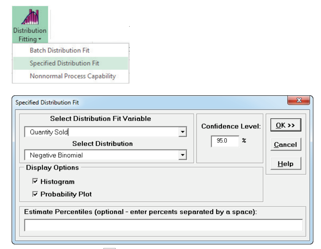
Optional Specified Distribution Fit analysis: This is a detailed
view of the distribution fit for a specified distribution with:
Histogram and Probability
Plot.
Parameter estimates, standard errors (SE Estimate)
and confidence intervals for parameter estimates.
o Note that percentiles are computed using the
distribution and estimated parameters, not empirical data.
Standard errors and confidence intervals for the
percentile values
Model Summary and Goodness-of-Fit statistics.
Select DiscoverSim > Distribution Fitting >
Specified
Distribution Fit:
Using the default settings as shown, click
OK. This produces a detailed distribution fit report for
Quantity Sold using the Negative Binomial distribution:
Now we will apply specified distribution fitting to Price and Variable
Cost. Repeat the above steps using the default best fit distributions to
produce a detailed distribution fit report:
The detailed distribution analysis clearly shows that we have a
good fit for all 3 variables. Now we will use the stored
distribution fits to create a DiscoverSim model.
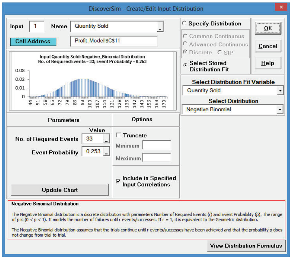
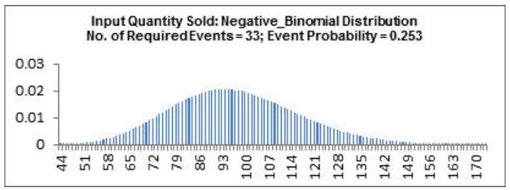
Select Profit_Model sheet. Click on cell C11 to
specify the Input Distribution for Quantity Sold. Select DiscoverSim
> Input Distribution.
Click Select Stored Distribution Fit. We will use the default variable
Quantity Sold for Select Distribution Fit Variable and
Negative Binomial for
Select Distribution. The parameter values for
Number of Required Events and Event Probability are
automatically populated from the distribution fit results for
Quantity Sold.
Enter QuantitySold as the Input Name.
Click Update Chart. The completed Create/Edit Input Distribution dialog
is shown below:
Click OK. Hover the cursor on cell
C11 in the Profit_Model sheet to view the DiscoverSim
graphical comment showing the distribution and parameter values:
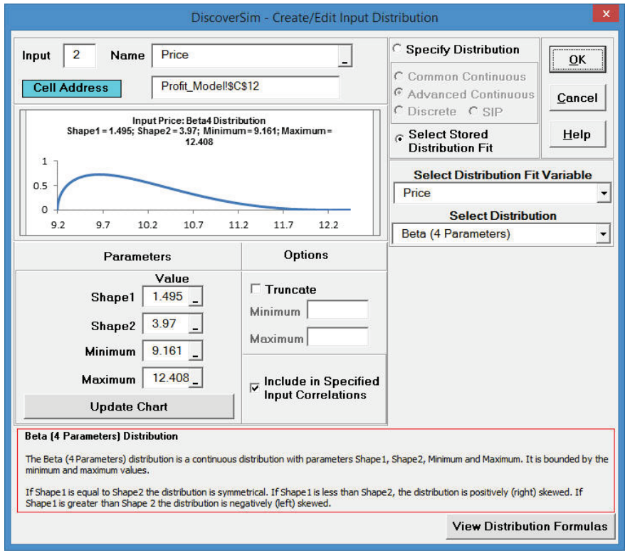
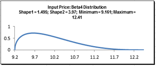
Click on cell C12 to specify the Input Distribution for Price.
Select DiscoverSim > Input Distribution.
Click Select Stored Distribution Fit. Select the variable
Price for
Select Distribution Fit Variable and the default
Beta (4 Parameters) for
Select Distribution. The parameter values for this distribution are
automatically populated from the distribution fit results for
Price.
Enter Price as the Input Name.
Click Update Chart. The completed Create/Edit Input Distribution dialog
is shown below:
Click OK. Hover the cursor on cell
C12 in the Profit_Model sheet to view the DiscoverSim
graphical comment showing the distribution and parameter values:
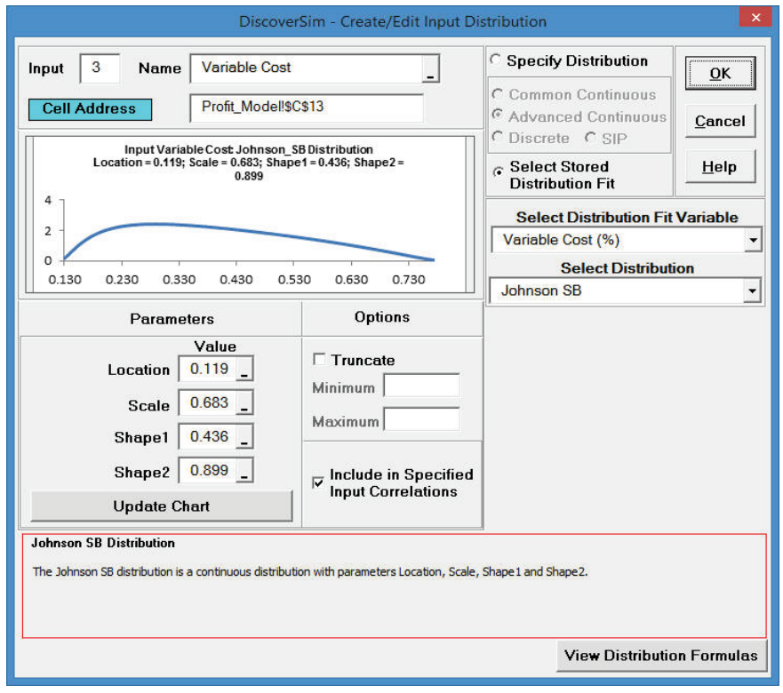
Click on cell C13 to specify the Input Distribution for
Variable Cost. Select
DiscoverSim > Input Distribution.
Click Select Stored Distribution Fit. Select
Variable Cost for
Select Distribution Fit Variable and the default
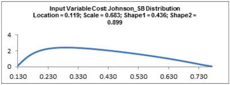
Johnson SB for Select Distribution. The parameter values for
this distribution are automatically populated from the distribution fit results for
Variable Cost.
Enter Variable Cost as the Input Name.
Click Update Chart. The completed Create/Edit Input Distribution dialog
is shown below:
Click OK. Hover the cursor on cell
C13 in the Profit_Model sheet to view the DiscoverSim
graphical comment showing the distribution and parameter values:
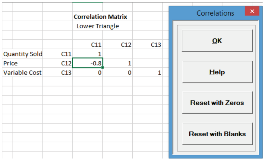
Now we will specify the correlation between the inputs Quantity Sold and Price. Select
DiscoverSim > Correlations:
As discussed above, the Spearman Rank correlation between Quantity and Price is -.8.
This negative correlation is expected: as order quantity increases, unit price
decreases. Enter the value -.8 in the column
Price, row Quantity and press Enter.
Tips: It is not necessary
to enter a correlation value in the upper triangle. The lower
triangle specifies the correlations so any value entered in the
upper will be ignored. The diagonal of 1s should not be altered.
Reset with Zeros clears any specified correlations
in the lower triangle and replaces them with zeros. Reset
with Blanks
clears any correlations in the lower triangle and replaces them with
blanks. This is useful if you wish to then specify correlations
between inputs without the constraint of requiring independence on
the other inputs.
Click OK.
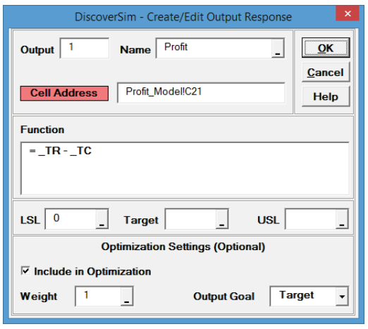
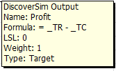
Now we will specify the Profit model output. Click on cell
C21. Select DiscoverSim > Output
Response:
Enter the output Name as Profit. Enter the Lower Specification Limit
(LSL) as 0. The
Include in Optomization,
Weight and OutputGoal settings are
used only for multiple response optimization, so do not need to be modified in this
example.
Click OK.
Hover the cursor on cell C21 to view the DiscoverSim Output
information.
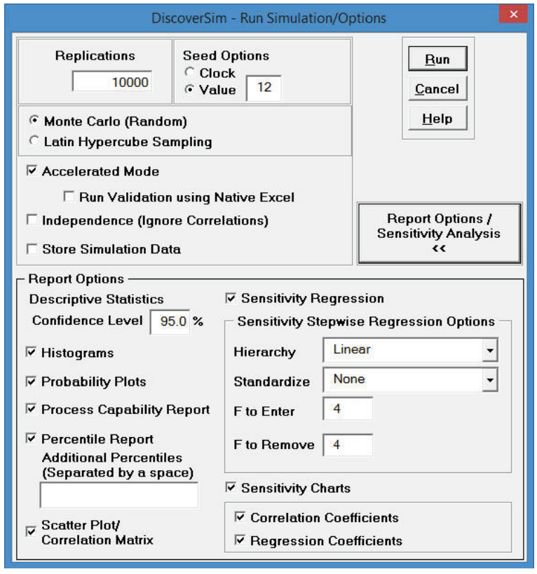
Select DiscoverSim > Run Simulation:
Click Report Options/Sensitivity Analysis. Check Percentile
Report, Scatter Plot/Correlation Matrix,
Sensitivity Regression Analysis, Sensitivity Charts -
Correlation Coefficients and Regression Coefficients. Select
Seed Value and enter 12 as shown, in order to replicate the
simulation results given below (note that 64 bit DiscoverSim will show slightly
different results).
Click Run
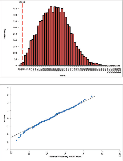
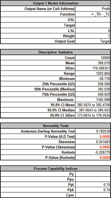
The DiscoverSim Output Report shows a histogram, normal probability plot, descriptive
statistics, process capability indices, a percentile report and a percentile process
capability report:
From the histogram and detailed report we see that typically we should expect a positive
daily profit, but the variation is large. The likelihood of profit loss is approximately
0.20% (see
Actual Performance (Empirical): %Total (out of spec). Note that the
expected loss of 1.36% assumes a normal distribution, so that is not applicable here
because the output distribution is not normal (Anderson-Darling p-value is much less
than .05).
Note: If Seed is set to Clock, there will be slight
differences in the reported values with every simulation run due to a different starting
seed value derived from the system clock.
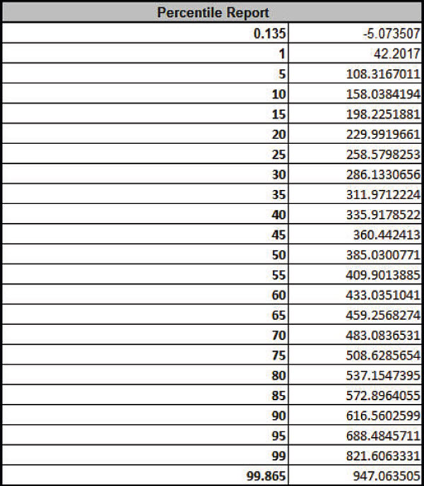
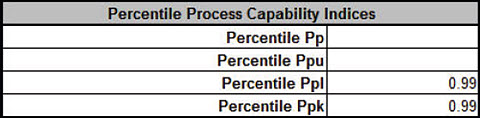
Tip: Percentile Process Capability Indices for non-normal data can be
calculated from the Percentile Report as follows:
Since we only have a lower specification limit (LSL = 0), Percentile Ppl is calculated
as: Percentile Ppl = (385.03 - 0) / (385.33 - (-5.07))
= 0.99
Optional Nonnormal Process Capability Analysis: DiscoverSim Version 2.1
now includes
Nonnormal Process Capability with Distribution
Fitting. To utilize this stand-alone feature for the Profit data, perform
the following steps:
Click Run Simulation, select Store Simulation
Data, click
Run.
Select DSim Data sheet, select Profit column
(D1:D10001).
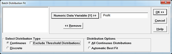
Select Distribution Fitting > Batch Distribution Fit,
click Next, select Profit, uncheck Exclude
Threshold Distributions:
Click OK. The batch fit will take approximately 1-2 minutes
due to the large dataset and inclusion of Threshold distributions.
The best fit distribution is Generalized Gamma with Threshold. Unfortunately,
it is not a good fit to the data with the AD P-Value < .001, but we will
proceed for demonstration purposes. Select Distribution Fitting >
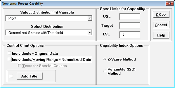
Nonnormal Process Capability.
Select Profit. Enter LSL = 0. The best fit
distribution is selected as Generalized Gamma with Threshold. Uncheck
Control Chart Options.
Click OK. The Ppk using Generalized Gamma is 0.95 which, even
though a poor fit, is closer to the above Percentile Ppk value of 0.99 than the
normal distribution Ppk of .74.
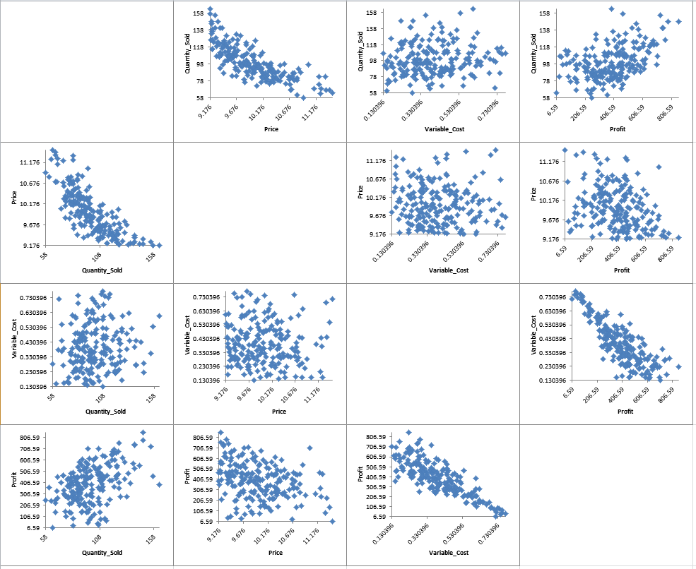
Click on the Scatter Plot Matrix sheet to view the
Input-Output relationships graphically:
Here we see the negative correlation that was specified between the inputs Price and
Quantity Sold, as well as the strong negative correlation between Variable Cost and
Profit.
Click on the Correlation Matrix sheet to view the Input-Output
correlations numerically:
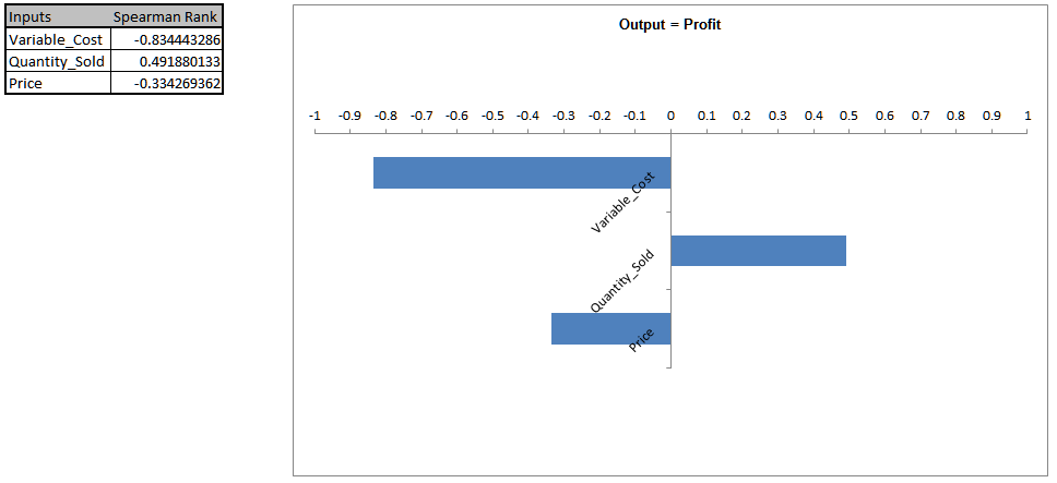
In order to increase profit (and reduce the variation), we need to understand what is
driving profit, i.e., the key X factor. To do this we will look at the sensitivity
charts. Click on the
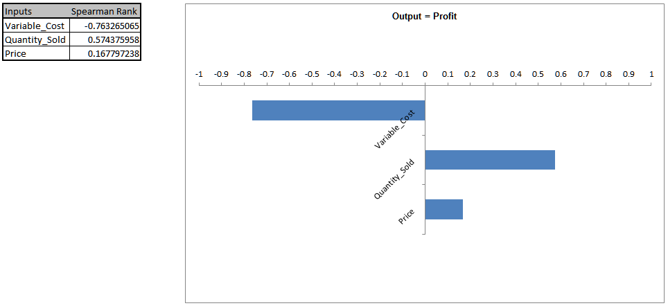
Sensitivity Chart sheet:
Here we see that Variable Cost is the dominant input factor affecting Profit with a
negative correlation (lower variable cost means higher profit). The next step would then
be to find ways to minimize the variable cost (and reduce the variation of variable
cost). Quantity Sold is the second important input factor. It is interesting to note
that Price is the least important factor in this Profit simulation model.
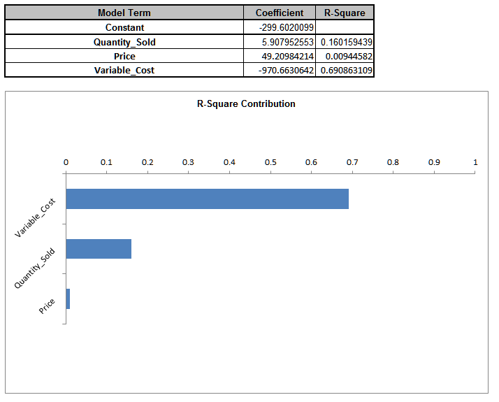
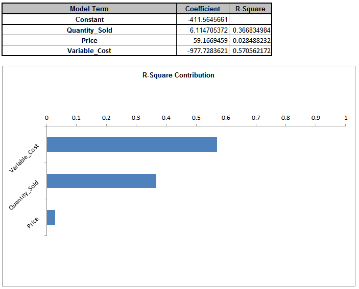
To view R-Squared percent contribution to variation, click on the
Sensitivity Regression sheet:
When strong correlations are present in the inputs, Sensitivity Correlation Analysis and
Sensitivity Regression Analysis may be misleading, so it is recommended that the
simulation be rerun with
Independence (Ignore Correlations) checked to validate the sensitivity
results:
In this case the input factor prioritization remains the same, but Price shows a small
positive correlation rather than negative.
The revised R-Square Percent Contribution report is shown below:


 to change it or select
Use Entire Data Table to automatically select the data.
to change it or select
Use Entire Data Table to automatically select the data.