Overview of Basic Design of Experiments (DOE) Templates
The DOE templates are similar to the other SigmaXL templates: simply
enter the inputs and resulting outputs are produced immediately. The DOE templates provide
common 2-level designs for 2 to 5 factors. These basic templates are ideal for training, but
use
SigmaXL > Design of Experiments > 2-Level Factorial/Screening Designs
to accommodate up to 19 factors with randomization, replication and blocking.
Click SigmaXL > Design of Experiments > Basic DOE Templates
to access these templates:
Two-Factor, 4-Run, Full-Factorial
Three-Factor, 4-Run, Half-Fraction, Res III
Three-Factor, 8-Run, Full-Factorial
Four-Factor, 8-Run, Half-Fraction, Res IV
Four-Factor, 16-Run, Full-Factorial
Five-Factor, 8-Run, Quarter-Fraction, Res III
Five-Factor, 16-Run, Half-Fraction, Res V
After entering the template data, main effects and interaction plots may be created by
clicking
SigmaXL > Basic DOE Templates > Main Effects & Interaction Plots.
The DOE template must be the active worksheet.
DOE Templates are protected worksheets by default, but this may be modified by
clicking
SigmaXL > Help > Unprotect Worksheet.
Advanced analysis is available, but this requires that you unprotect the DOE worksheet. The
following example shows how to use Excels Equation Solver and SigmaXLs Multiple Regression
in conjunction with a DOE template.
Caution: If you unprotect the worksheet, do not change the worksheet title
(e.g.
Three-Factor, Two-Level, 8-Run, Full-Factorial Design of Experiments). This
title is used by the Main Effects & Interaction Plots to determine appropriate analysis.
Also, do not modify any cells with formulas.
Three Factor Full Factorial Example Using DOE Template
Open the file DOE Example - Robust Cake.xlsx. This is a Robust Cake
Experiment adapted from the Video Designing Industrial Experiments, by Box, Bisgaard and
Fung.
The response is Taste Score (on a scale of 1-7 where 1 is "awful" and 7 is "delicious").
The five Outer Array Reps have different Cooking Time and Temperature Conditions.
The goal is to Maximize Mean and Minimize StDev of the Taste Score.
The X factors are Flour, Butter, and Egg. Actual low and high settings are not given in
the video, so we will use coded -1 and +1 values. We are looking for a combination of
Flour, Butter, and Egg that will not only taste good, but consistently taste good over a
wide range of Cooking Time and Temperature conditions.
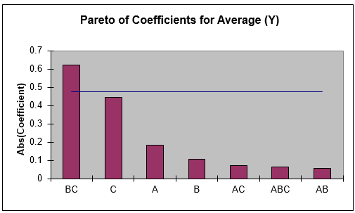
Scroll down to view the Pareto of Abs. Coefficients for Average (Y).
The BC (Butter * Egg) interaction is clearly the dominant factor. The bars above the 95%
confidence blue line indicate the factors that are statistically significant; in this
case only BC is significant. Keep in mind that this is an initial analysis. Later, we
will show how to do a more powerful Multiple Regression analysis on this data. (Also,
the Rule of Hierarchy states that if an interaction is significant, we must include the
main effects in the model used.)
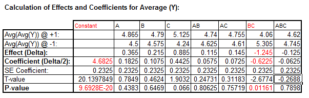
The significant BC interaction is also highlighted in red in the table of Effects and
Coefficients:
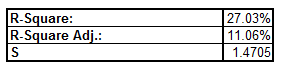
The R-Square value is given as 27%. This is very poor for a Designed Experiment.
Typically, we would like to see a minimum of 50%, with > 80% desirable.
The reason for the
poor R-square value is the wide range of values over the Cooking Temperature and Time
conditions. In a robust experiment like this, it is more appropriate to analyze the mean
response as an individual value rather than as five replicate values. The Standard
Deviation as a separate response will also be of interest.
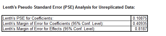
If the Responses are replicated, SigmaXL draws the blue line on the Pareto Chart using
an estimate of experimental error from the replicates. If there are no replicates, an
estimate called Lenths Pseudo Standard Error is used.
If the 95% Confidence line for coefficients were to be drawn using Lenths method, the
value would be 0.409 as given in the table:
This would show factor C as
significant.
Scroll down to view the Pareto of Coefficients for StdDev(Y).
The A (Flour) main effect is clearly the dominant factor, but it does not initially
appear to be statistically significant (based on Lenths method). Later, we will show
how to do a more powerful Regression analysis on this data.
The Pareto chart is a powerful tool to display the relative importance of the main
effects and interactions, but it does not tell us about the direction of influence. To
see this, we must look at the main effects and interaction plots. Click
SigmaXL > Basic DOE Templates > Main Effects & Interaction
Plots. The resulting plots are shown below:
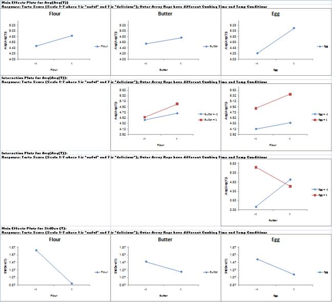
The Butter*Egg two-factor interaction is very prominent here. Looking at only the Main
Effects plots would lead us to conclude that the optimum settings to maximize the
average taste score would be Butter = +1, and Egg = +1, but the interaction plot tells a
very different story. The correct optimum settings to maximize the taste score is Butter
= -1 and Egg = +1.
Since Flour was the most prominent factor in the Standard Deviation Pareto, looking at
the Main Effects plots for StdDev, we would set Flour = +1 to minimize the variability
in taste scores. The significance of this result will be demonstrated using Regression
analysis.
Click on the Sheet
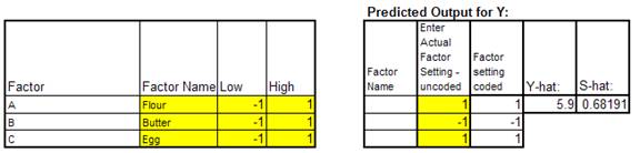
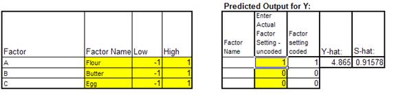
Three-Factor 8-Run DOE. At the Predicted Output for Y,
enter
Flour = 1, Butter = -1, Egg = 1 as shown:
The predicted average (Y-hat) taste score
is 5.9 with a predicted standard deviation (S-hat) of 0.68. Note that this prediction
equation includes all main effects, two-way interaction, and the three-way interaction.
Multiple Regression and Excel Solver (Advanced Topics):
In order to run Multiple Regression analysis we will need to unprotect the
worksheet. Click
SigmaXL > Help > Unprotect Worksheet.
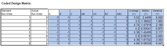
In the Coded Design Matrix, highlight columns A to ABC, and the
calculated responses as shown:
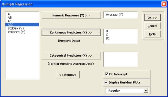
Select Average (Y), click Numeric Response (Y) >>;
holding the CTRL key, select
B, C, and BC; click Continuous Predictors (X)
>> as shown:
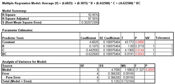
Click OK. The resulting regression report is shown:
Note that the R-square value of 92.85% is much higher than the earlier result of
27%. This is due to our modeling the mean response value rather than considering all
data in the outer array. Note also that the C main effect now appears as
significant.
Click on the Sheet
Three-Factor 8-Run DOE.
With the Coded Design Matrix highlighted as before, click
SigmaXL > Statistical Tools > Regression > Multiple
Regression. Click
Next.
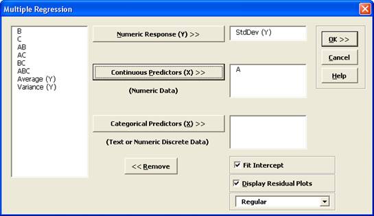
Select StdDev (Y), click Numeric Response (Y) >>;
select
A, click Continuous Predictors (X) >>
as shown:
Click
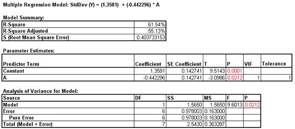
OK. The resulting regression report is shown:
Note that Factor A (Flour) now shows as a statistically significant factor affecting
the Standard Deviation of Taste Score.
Now we will use Excels Equation Solver to verify the optimum settings determined
using the Main Effects and Interaction Plots.
Click on the Sheet
Three-Factor 8-Run DOE. At the Predicted Output for
Y, enter 1 for
Flour. We are setting this as a constraint, because Flour = +1 minimizes
the Standard Deviation. Reset the
Butter and Egg to 0 as shown:
Click
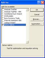
Tools > Add-Ins. Ensure that the
Solver Add-in is checked. If the Solver Add-in does not appear in
the Add-ins available list, you will need to re-install Excel to include all
add-ins.
Click
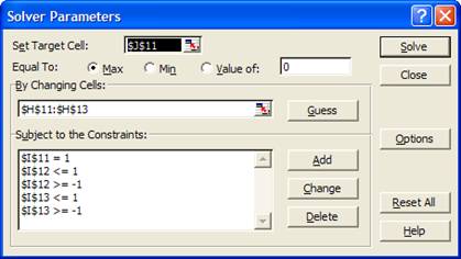
OK. Click Tools > Solver. Set the
Solver Parameters as shown:
Cell J11 is the Y-hat, predicted average taste score. Solver will try to maximize
this value. Cells H11 to H13 are the Actual Factor Settings to be changed. Cells I11
to I13 are the Coded Factor settings where the following constraints are given:
I11=1; I12 >= -1; I12 <= 1; I13 >= -1; I13 <=1.
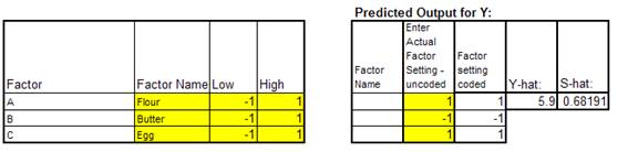
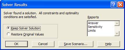
Click
Solve. The solver results are given in the
Predicted Output for Y as Butter = -1 and
Egg = 1.