Example 1: Advanced 2-Level Factorial/Screening Design with Augment - Add Axial Points - Cake Bake

We will illustrate the use of an Advanced 2-Level Factorial/Screening Design with the factorial + center point portion of the response surface layer cake baking experiment given in Part D - Design and Analysis of Response Surface Experiment - Cake Bake. . The response variable is Taste Score (on a scale of 1-7 where 1 is "awful" and 7 is "delicious"). Average scores for a panel of tasters have been recorded. The Continuous Factors are A: Bake Time (20 to 40 minutes) and B: Oven Temperature (350 to 400 F). The experiment goal is to find the settings that maximize taste score.

After analysis, the design will be augmented to add axial points making it a response surface design.

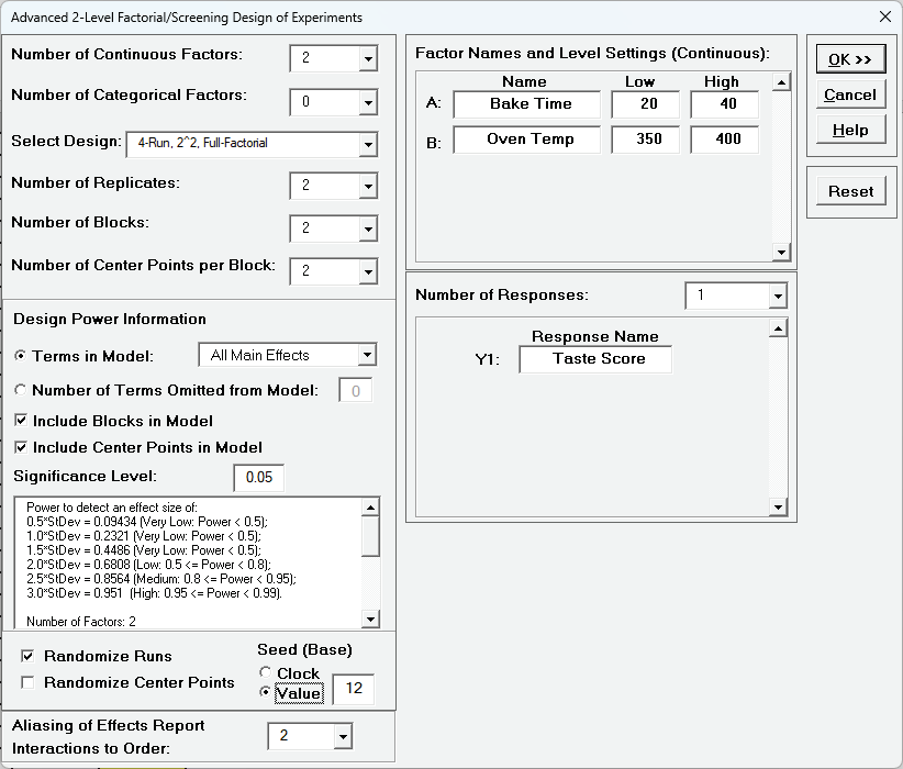
1. Click SigmaXL > Design of Experiments > Advanced Design of Experiments: 2-Level Factorial/Screening > 2-Level Factorial/Screening Designs. The default dialog design is given as:






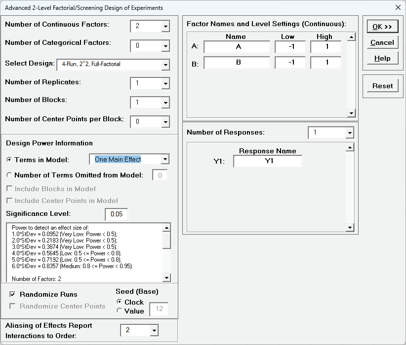
First, we will look at the Design Power Information for the default settings. The report is given as:






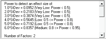
This initial 2 Factor 4 Run design has very low power to detect a large effect size of 3.0*StDev and only medium power to detect an extreme effect size of 6.0*StDev.




Scroll down to view the full report.






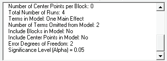
With Terms in Modelas One Main Effect, Error Degrees of Freedom = 2. Typically, we want Terms in Model as All Main Effects but here that only gives Error Degrees of Freedom = 1. If Terms in Model l is selected as ME + 2-Way Interactions, then Error Degrees of Freedom = 0 and power cannot be calculated.

2. Select Number of Replicates = 2, Number of Blocks = 2, Number of Center Points per Block = 2 and Design Power Information - Terms in Model as All Main Effects.






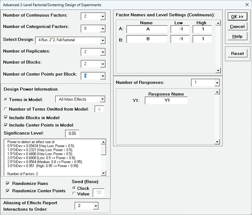
This design now has medium power to detect an effect size = 2.5*StDev (with error degrees of freedom = 7), so is a dramatic improvement over the single replicate case. This is the design that we will use for the cake bake example as it matches the factorial portion (plus center points) of the response surface design.

3. Enter Factor Names and Level Settings, Response Name as shown. Uncheck Randomize Center Points, select Seed (Base) - Value with default 12. Aliasing of Effects Report - Interactions to Order r has default 2 but is not relevant here as this is a full factorial design.





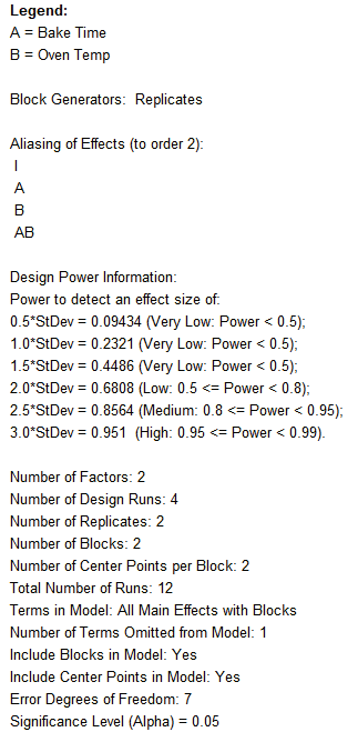
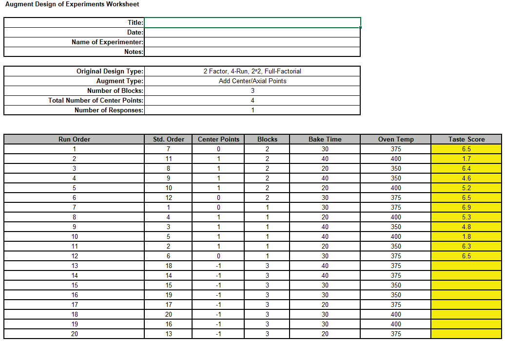
4. Click OK. The following Design of Experiments Worksheet is produced including the Legend, Block Generators, Aliasing of Effects and Design Power Information:








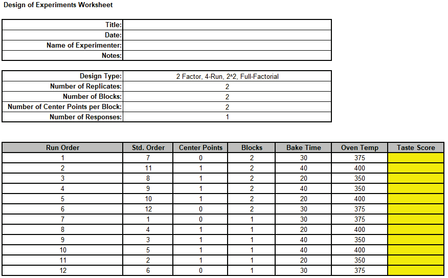
Note that by unchecking Randomize Center Points,the center points are (approximately) equally spaced within a block. With two center points they are the first and last runs within the block. If there are 3, then first, middle and last runs are used.




Since Randomize Runsis checked, the non-center points are randomized within the block. Note that block number is also randomized. Using the fixed seed = 12, means that the random run order will always be the same, which is useful for instructional purposes.




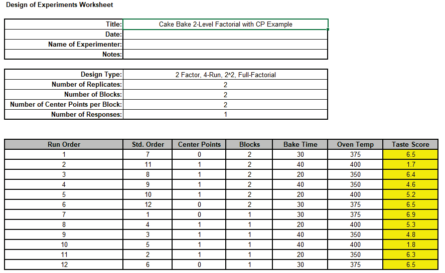
5. Open the file Advanced 2-Level Factorial Example - Cake Bake.xlsx This has the design worksheet populated with Taste Score values.






6. Click SigmaXL > Design of Experiments > Advanced Design of Experiments: 2-Level Factorial/Screening > Analyze 2-Level Factorial/Screening Design.

7. Select Responses and Model Terms as shown with Term Generator as ME + 2-Way Interactions. Uncheck Include Center Points:






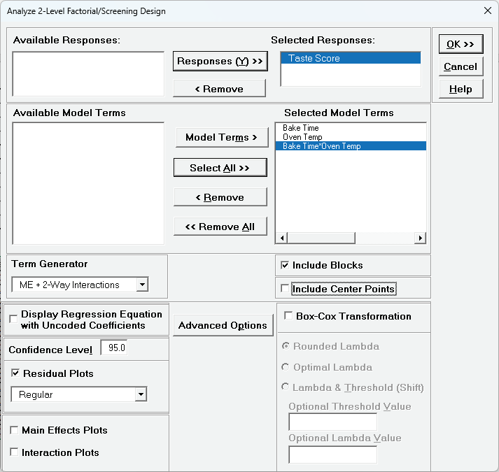
Include Center Points is unchecked because we want to be able to clearly see the influence of the center points in the Residual Plots. We will redo the analysis later with Include Center Points checked. Advanced Optionsare the same as those used in Advanced Multiple Regression. We will use the defaults.

8. Click OK.






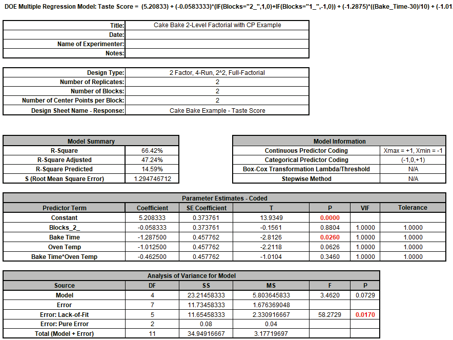
Note the significant Error: Lack-of-Fit with P-Value = 0.017. Only Bake Time is significant, and the R-Square, R-Square Adjusted and R-Square Predicted are low.

9. Click on the Residuals Taste Score sheet.






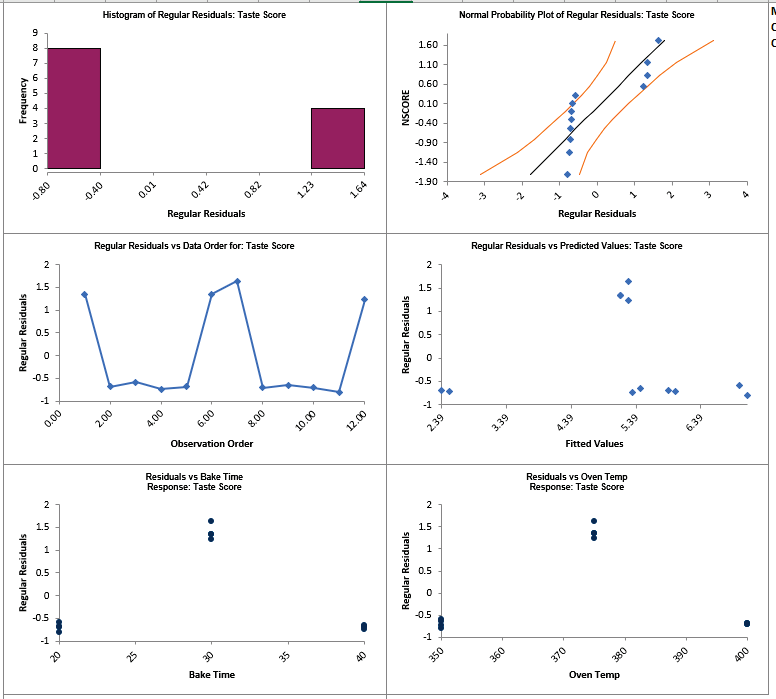
The residual plots show obvious non-random, non-normal patterns, and in particular the Residuals vs Bake Time and Residuals vs Oven Temp show strong curvature.

10. Now we will re-analyze the experiment and include center points in the model. Click Recall Last Dialog (or press F3) (or press Check Include Center Points.






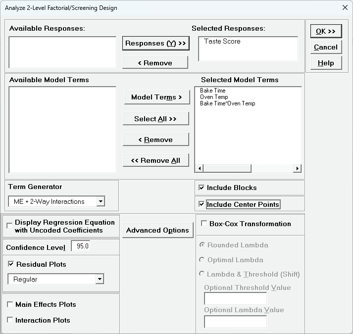
11. Click OK.





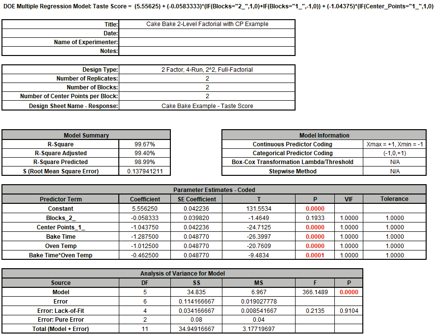
All model terms except Blocks are significant, the R-Square values are high and there is no Significant Lack of Fit (with P-Value = 0.91). The Residual Plots also show no obvious patterns.




Note however that the Center Points term is significant so this indicates significant curvature or quadratic effects. This means that we cannot use the model as is to make predictions, we need to specify quadratic terms for Bake Time and Oven Temp. The current full-factorial + center point design does not permit these quadratic terms to be added as they would be confounded. We need to augment the design to add axial points, effectively converting this design into a response surface design.




We could also refit the model withInclude Blocksunchecked but we will not do so here.

12. Click on sheet Cake Bake Example in Advanced 2-Level Factorial Example - Cake Bake.xlsx.

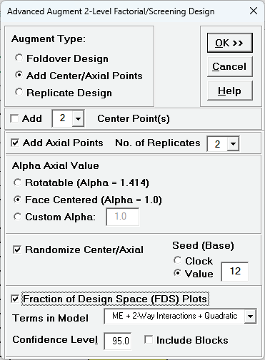
13. Click on sheet SigmaXL > Design of Experiments > Advanced Design of Experiments: Augment 2-Level Factorial/Screening > Augment Design. The default dialog design is given as Augment Type: Foldover Design Select Augment Type: Add Center/Axial Points.

14. Uncheck Add Center Points since we already have center points in the original design. Use the default checked Add Axial Points No. of Replicates = 2 which matches the number of replicates in the factorial design. Select Face Centered (Alpha = 1.0) to match the original Cake Bake RSM design. Check Randomize Center/Axial, select Seed (Base) Value = 12, and check Fraction of Design Space (FDS) Plots with options selected as shown:





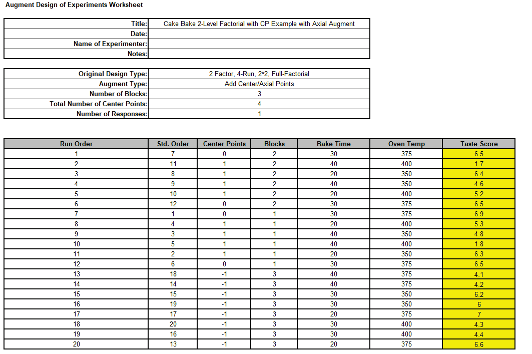
15. Click OK. The worksheet augments the original factorial design with 8 new axial runs randomized within a block, i.e., 4 axial runs replicated twice.





The Fraction of Design Space (FDS) Plots and report are given as:







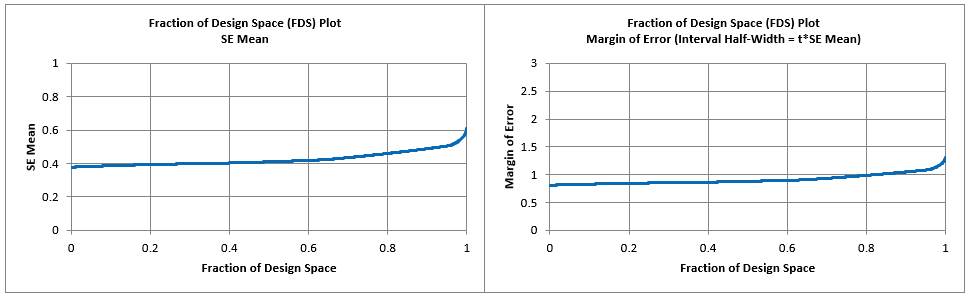
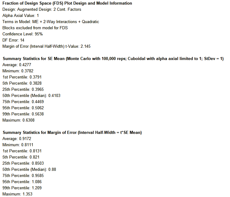
For details on FDS Plots, see the Appendix: Fraction of Design Space (FDS) Plots. See also Example 3: Evaluating Response Surface and Optimal Designs with the Fraction of Design Space (FDS) Plot.




The Margin of Error (Interval Half-Width) at the 95th Percentile (i.e. 95% of the design space) is 1.086. We then multiply this by the estimate of the model standard deviation of 0.138 given in the factorial portion to obtain a Margin of Error for Taste Score = 1.086 * 0.138 = 0.15. Given that the Taste Score is on a 1 to 7 scale this is an acceptable margin of error for prediction.

16. Open the file Advanced 2-Level Factorial Example - Cake Bake with Axial Augment.xlsx which has the augmented design worksheet populated with Taste Score values. Click on the sheet Cake Bake Axial Augment.





17. Click SigmaXL > Design of Experiments > Advanced Design of Experiments: Augment 2-Level Factorial/Screening > Analyze Augmented Design.

18. Select Responses and Model Terms as shown with Term Generator as ME + 2-Way Interactions + Quadratic. Quadratic terms can now be estimated because we augmented the factorial design with axial points. Check ADisplay Regression Equation with Uncoded Coefficients We will not modify Advanced Options Leave Include Blocks unchecked.






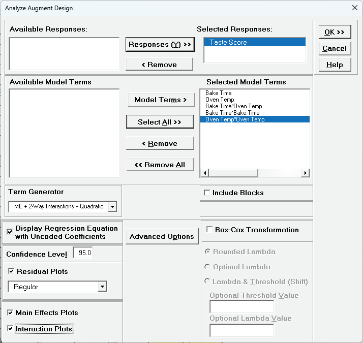
19. Click OK. This gives a Multiple Regression report that is identical to the one given earlier in Analysis of Response Surface Experiment - Cake Bake with Advanced Multiple Regression (except for the report header information):






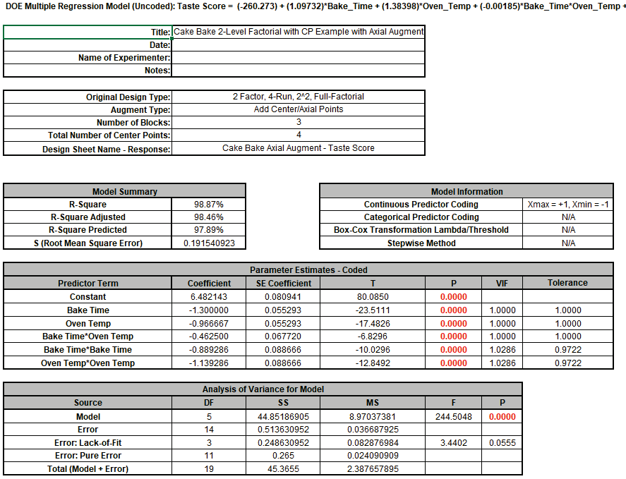
We will not review the regression report, residuals or main effects/interaction plots here as that was already done in the earlier analysis, but we will review the use of the Predicted Response Calculator, Optimize and Contour/Surface Plots.

20. Scroll to the Predicted Response Calculator Enter Bake Time = 23, Oven Temp = 368 to predict Taste Score with the 95% confidence interval for the long term mean and 95% prediction interval for individual values:






Note the formula at cell L14is an Excel formula with uncoded coefficients and range names that are scoped to the sheet not the workbook. If coded coefficients are desired rerun the above analysis withDisplay Regression Equation with Uncoded Coefficientsunchecked.The Margin of Error (Interval Half-Width) is 7.21 - 7.05 = 0.16, which is close to what we estimated using the FDS Plot. Given that the Taste Score is on a 1 to 7 scale this is an acceptable margin of error for prediction.

21. Next, we will use SigmaXL's built in Optimizer. Scroll to view the Optimize Options:





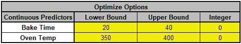
Here we can constrain the lower and upper bounds of the continuous predictors, but we will leave the default settings as is, which are obtained from the minimum and maximum of the predictor values.

22. Scroll back to view the Goal setting and Optimize button. Specify Goal = Maximize.





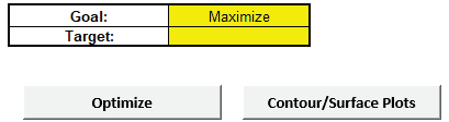
The optimizer uses Multistart Nelder-Mead Simplex to solve for the desired response goal with given bounds. For more information see the Appendix: Single Response Optimization. Single Response Optimization.

23. Click Optimize. The response solution and prompt to paste values into the Input Settings of the Predicted Response Calculator is given:





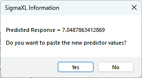
24. Click Yes to paste the values.





25. Next, we will create a Contour/Surface Plot. Click the Contour/Surface Plots button.

26. A new sheet is created, AdvAug1 - Contour that displays the plots:





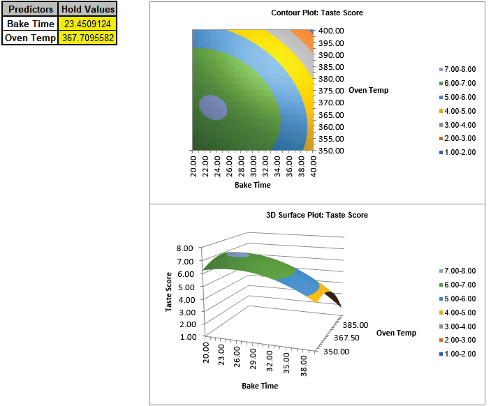
This matches the Contour and Surface Plots given in the previous analysis.




The table with the Hold Values,gives the values used to hold a predictor constant if it is not in the plot, so is not applicable here with only one plot based on the two continuous predictors.




Tip:Use the contour/surface plots in conjunction with the predicted response calculator to determine optimal settings.