Example 5: Evaluating Response Surface Designs with the Fraction of Design Space (FDS) Plot

Power analysis is very useful to assist in the design of 2 level factorial and fractional-factorial experiments. In a similar manner, the Fraction of Design Space (FDS) Plot assists the practitioner to select and right size their multi-level response surface and optimal designs. The FDS Plot was introduced by Zahran, Anderson-Cook and Myers [10].




The FDS Plot provides a visual representation of how well the design covers the experimental space and helps in assessing the precision of predictions that can be made from the design. This can be used to compare and select number of replicates, number of center points, Central Composite alpha axial value, Central Composite vs Box-Behnken and optimality criterion. The FDS Plot will show Prediction Standard Error of the Mean (SE Mean) vs Fraction of Design Space and Margin of Error vs Fraction of Design Space.








When comparing FDS Plots, lower is better and flatter is better over the majority of the design space. If you know the process standard deviation you can use the Margin of Error plot to assess if the actual prediction error will be acceptable over the majority of the design space (typically use FDS = 80 to 95%).




The FDS Plot is produced prior to any data collection. Like the power calculations used in factorial designs, FDS assumes that the model standard deviation is 1. If the standard deviation is known, multiply the FDS Plot values by this standard deviation to get actual response units.




A model must be specified for FDS, typically that will be an RSM Quadratic model (Main Effects + 2- Way Interactions + Quadratic Terms) with 95% Confidence Level. The FDS Plots are computed using Monte Carlo simulation with a uniform distribution and coded values from -1 to +1, hence cuboidal. This occurs even for rotatable Central Composite designs which allows for comparison of FDS Plots across various design types. For formula details, see the Appendix:Fraction of Design Space (FDS) Plots.

SE Mean and Margin of Error are computed for 100,000 random values. These are sorted from smallest to largest and the results are plotted as SE Mean vs Fraction of Design Space and Margin of Error (Interval Half-Width) vs Fraction of Design Space using 1000 plot points.




Cake Bake RSM Example 1

This is the layer cake baking experiment revisited. The response variable is Taste Score (on a scale of 1-7 where 1 is "awful" and 7 is "delicious"). Average scores for a panel of tasters have been recorded. The X Factors are A: Bake Time (20 to 40 minutes) and B: Oven Temperature (350 to 400 F). The experiment is a 10-Run, Central Composite Design (CCD) with 2 Center Points, Face Centered with Alpha Axial = 1.0. We will first introduce the concept of the Fraction of Design Space Plot by analyzing this data and manually inputting values into the Predicted Response Calculator.

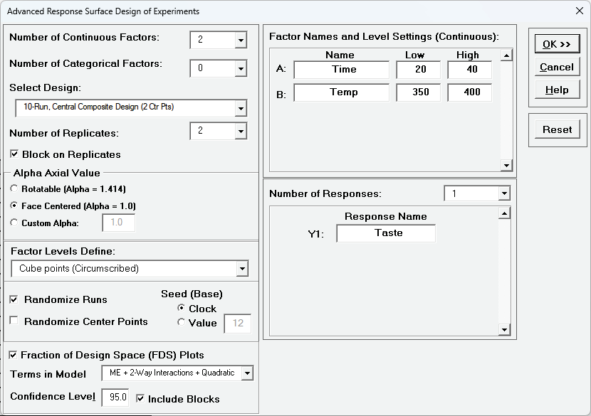
Cake Bake RSM Example 1 was created by clicking: SigmaXL > Design of Experiments > Advanced Design of Experiments: Response Surface > Response Surface Designs.







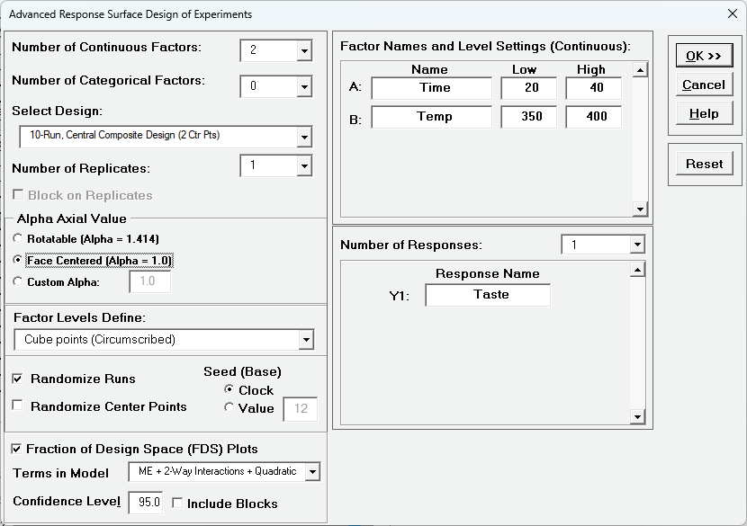
This is a 10 Run, Central Composite Design with 2 Center Points, Face Centered, and 1 Replicate. The FDS Plot uses a Quadratic Model with 95% Confidence Interval. Click OK.




Now open the file RSM FDS Example - Cake Bake.xlsx, Sheet Example 1. This is populated with the Taste Score response values.






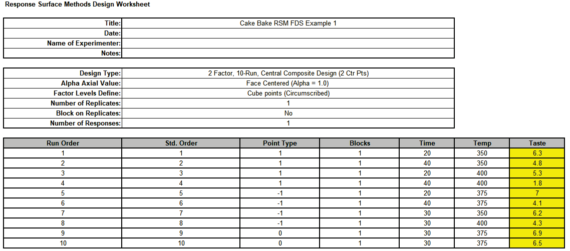
Runs are randomized in the actual experiment, but standard order is used for this demonstration.




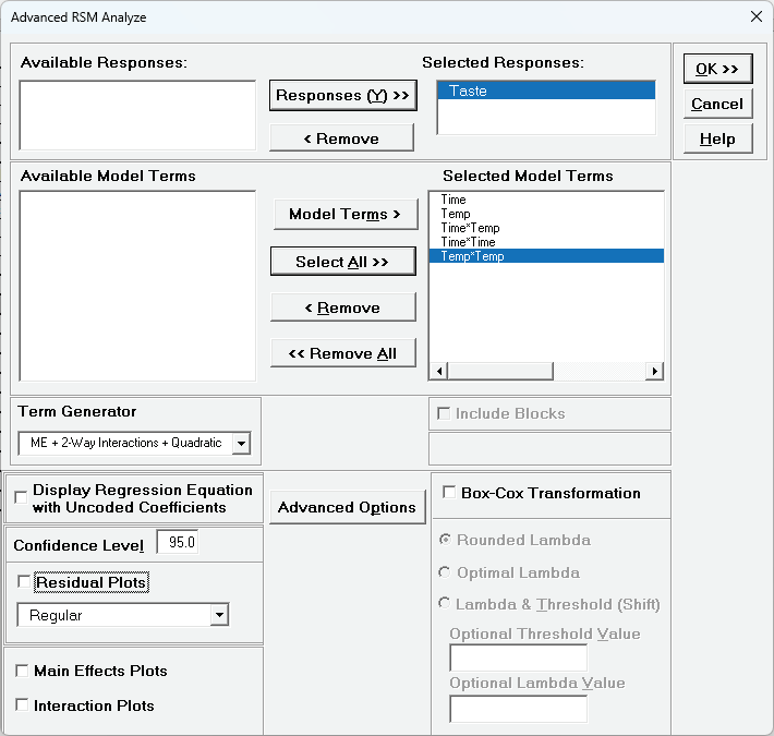
Click SigmaXL > Design of Experiments > Advanced Design of Experiments: Response Surface > Analyze Response Surface Design. Select Responses and Model Terms as shown. Uncheck Residual Plots.






Click OK.






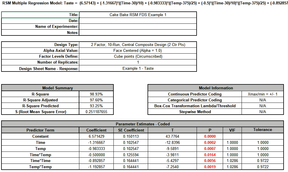
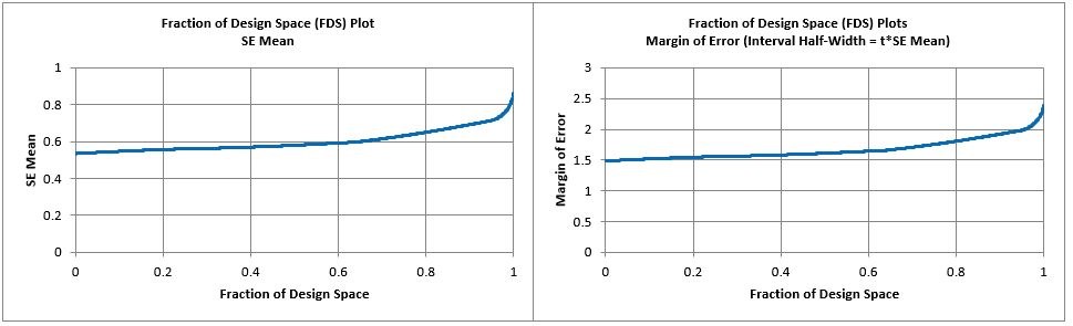
Scroll to the Predicted Response Calculator. Enter the center point values Time = 30 and Temp = 375. This gives a Predicted Response for Taste = 6.57 with a Standard Error = 0.15 and 95% CI = 6.15 to 6.99.






The Margin of Error (Interval Half-Width) is 6.99 - 6.57 = 0.42. This is a wide interval considering that the taste score is on a scale of 1 to 7.




Now enter Time = 20 and Temp = 350. This gives a Predicted Response for Taste = 6.29 with a Standard Error = 0.22 and 95% CI = 5.66 to 6.91






The Margin of Error (Interval Half-Width) is 6.91 - 6.29 = 0.62. This is an even wider interval than that obtained with the center points.




The Fraction of Design Space (FDS) Plot will repeat the above process 100,000 times using a uniform random number from 20 to 40 for Time and 350 to 400 for Temp. to obtain 100,000 SE and Half-Interval values. These are sorted from smallest to largest and the results are plotted as SE Mean vs Fraction of Design Space and Margin of Error (Interval Half-Width) vs Fraction of Design Space using 1000 plot points.




Hover the mouse cursor on the FDS plot to obtain values for any fraction of design space.





Smaller is better and flatter is better, over the majority of the design space.




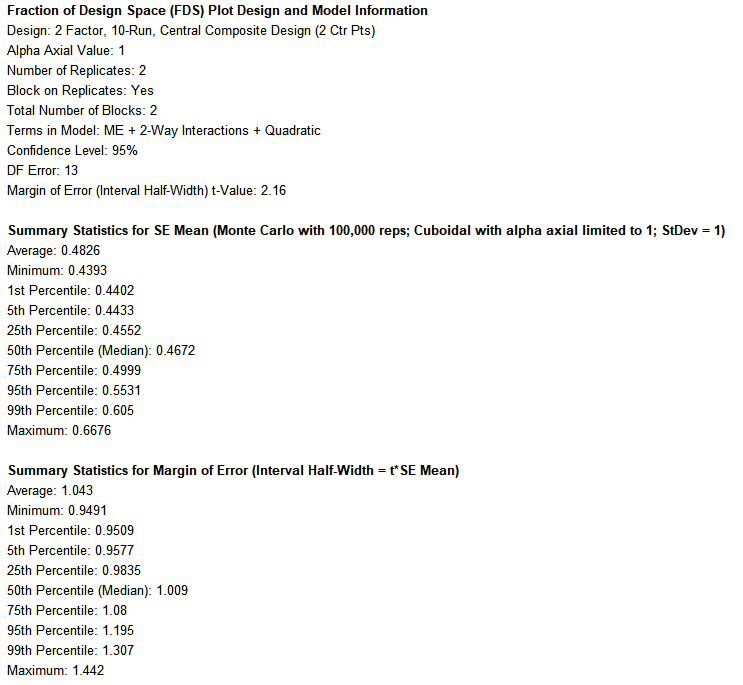
The FDS Summary Statistics complement the FDS Plot.








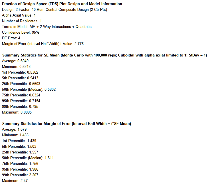
Looking at the 95th Percentile (i.e., 95% of the design space), we see that the SE Mean can be as large as .72 and the Margin of Error (Interval Half-Width) as large as 1.99.




To obtain units of Taste Score, we multiply by the model standard deviation: SE Mean = 0.72*0.25 = 0.18 and Half-Width = 1.99*0.25 = 0.5. As noted previously, this is a large margin of error considering that the taste score is on a 7-point scale.




Note that the Confidence Level of 95% applies to the Margin of Error. The 95th Percentile applies to the Fraction/Proportion of Design Space.




Since these percentiles are based on Monte Carlo simulation, slightly different results will be observed every time they are produced unless a fixed seed is used.




Cake Bake RSM Example 2

1. Cake Bake RSM Example 2 was created by clicking: SigmaXL > Design of Experiments > Advanced Design of Experiments: Response Surface > Response Surface Designs.











2. This is a 10 Run, Central Composite Design with 2 Center Points, Face Centered, 2 Replicates and Block on Replicates. The FDS Plot uses a Quadratic Model with 95% Confidence Interval and Blocks are included. Click OK.




3. Now open the file RSM FDS Example - Cake Bake.xlsx, Sheet Example 2. This is populated with the Taste Score response values.











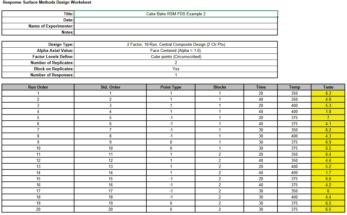
This has 2 Replicates of the previous Cake Bake design, with Block on Replicates. This will be used to demonstrate the impact that replicates have on the SE Mean and Margin of Error (Interval Half-Width).




4. Click SigmaXL > Design of Experiments > Advanced Design of Experiments: Response Surface > Analyze Response Surface Design. Select Responses and Model Terms as shown. Check Include Blocks. Uncheck Residual Plots.











5. Click OK.










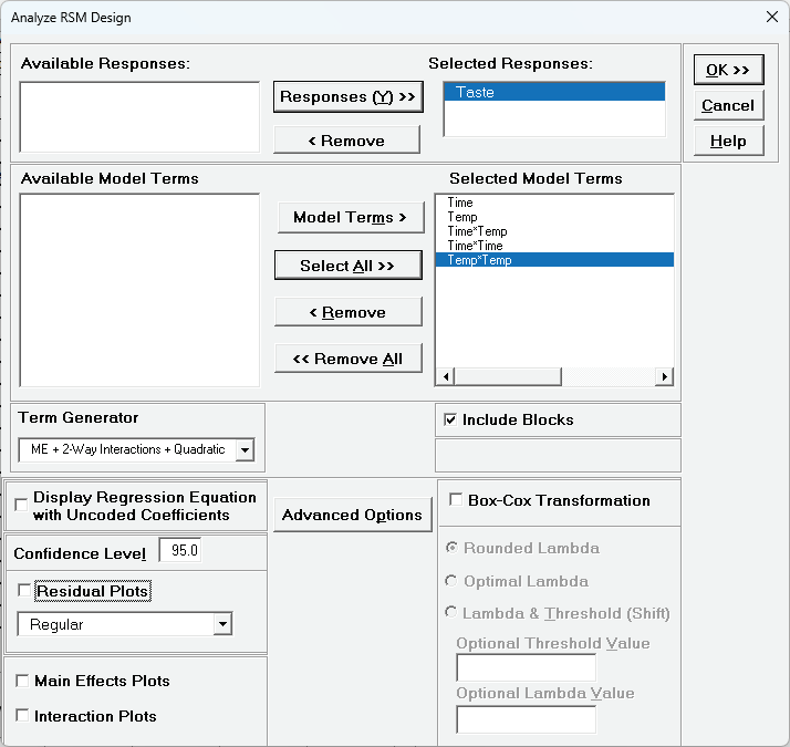
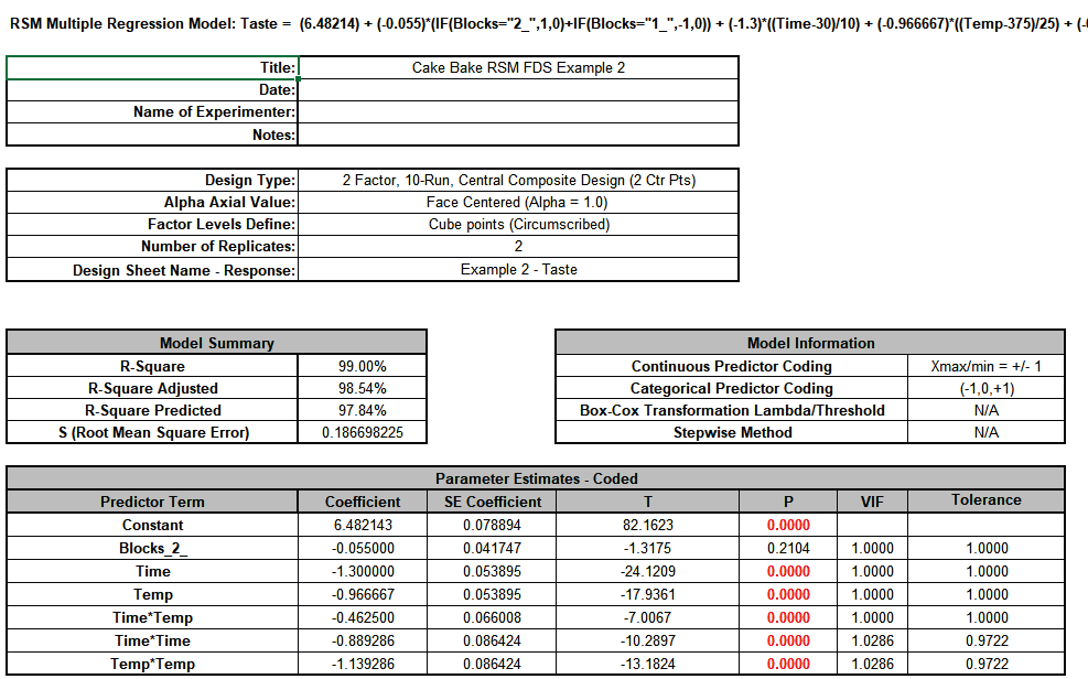
Since the Block term is insignificant, we will refit with Blocks removed from the model.



6. Click Recall SigmaXL Dialog and uncheck Include Blocks. Click OK.






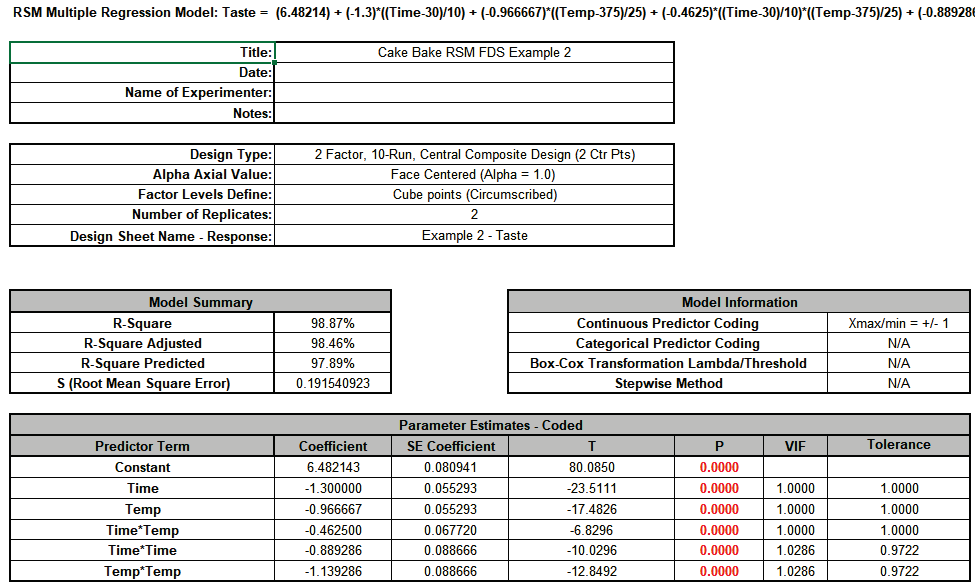
7. Scroll to the Predicted Response Calculator. Enter the center point values Time = 30 and Temp = 375. This gives a Predicted Response for Taste = 6.48 with a Standard Error = 0.08 and 95% CI = 6.31 to 6.66.







The Margin of Error (Interval Half-Width) is 6.66 - 6.48 = 0.18. This is a dramatic reduction from the previous value of 0.42 and is an acceptable interval for the 1-7 taste score.




8. Hover the mouse cursor on the FDS plot to obtain values for any fraction of design space.







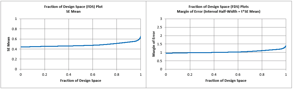
Smaller is better and flatter is better, over the majority of the design space.




9. The FDS Summary Statistics complement the FDS Plot.







Looking at the 95th Percentile (i.e., 95% of the design space), we see that the SE Mean can be as large as .55 and the Margin of Error (Interval Half-Width) as large as 1.2.




10. To obtain units of Taste Score, we multiply by the model standard deviation: SE Mean = 0.55*0.19 = 0.1 and Half-Width = 1.2*0.19 = 0.23.





11. As noted, this is an acceptable margin of error for the 1-7 taste score.





12. The FDS Plot for Example 2 included Blocks so could be redone without Blocks, but we will not do so here.





13. To create Overly FDS Plots, click SigmaXL > Design of Experiments > Advanced Design of Experiments: Overlay FDS Plots. Select FDS Plot Sheets and enter Legend names as shown:







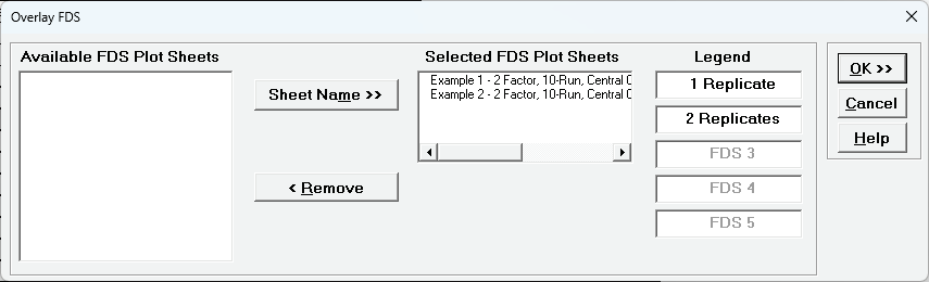
14. Click OK.







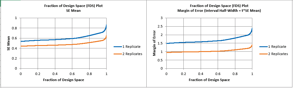
Here we can see a dramatic reduction in SE Mean and Margin of Error from the 2 Replicates vs 1 Replicate design!




Central Composite: Number of Center Points

15. Next, we will examine the effect of changing the number of Center Points in a Central Composite Design. Click SigmaXL > Design of Experiments > Advanced Design of Experiments: Response Surface > Response Surface Designs. Select Seed (Base) Value = 12.







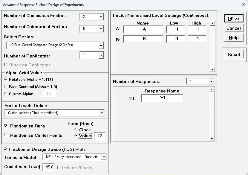
16. This is a 10 Run, Central Composite Design with 2 Center Points, Rotatable (Alpha = 1.414), 1 Replicate. The FDS Plot uses a Quadratic Model with Confidence Level = 95%. FDS will also use the Fixed Seed = 12 for replicable results. Click OK.





17. Click Recall SigmaXL Dialog. Select 13 Run, CCD, Uniform Precision (5 Ctr Pts).







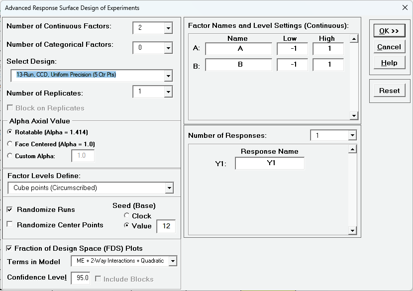
18. This is a 13 Run, Central Composite Design with 5 Center Points, Uniform Precision, Rotatable (Alpha = 1.414), and 1 Replicate. Click OK.





19. To create Overly FDS Plots, click SigmaXL > Design of Experiments > Advanced Design of Experiments: Overlay FDS Plots. Select FDS Plot Sheets and enter Legend names as shown:







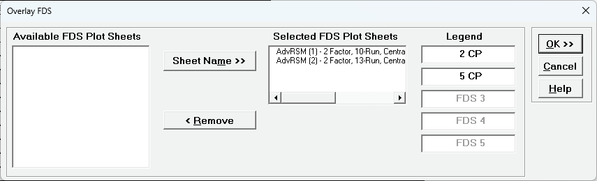
20. Click OK.







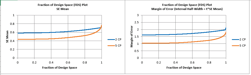
Here we can see a considerable reduction in SE Mean and Margin of Error from the 5 Center Points (5 CP) vs 2 Center Points (2 CP).




CCD Rotatable vs CCD Face Centered vs Box-Behnken

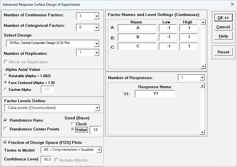
21. Now we will compare Central Composite Rotatable vs Central Composite Face Centered vs Box-Behnken designs. Click SigmaXL > Design of Experiments > Advanced Design of Experiments: Response Surface > Response Surface Designs. Select Number of Continuous Factors = 3, and Design: 16-Run, Central Composite Design (2 Ctr Pts), Seed (Base) Value = 12 and other options as shown:







22. This is a 3 Factor, 16 Run Central Composite Rotatable Design with Alpha = 1.682, 1 Replicate. The 16 Run CCD is selected for comparison to a 15 Run Box-Behnken. The FDS Plot uses a Quadratic Model with Confidence Level = 95%. FDS will also use the Fixed Seed = 12 for replicable results. Click OK.





23. Click Recall SigmaXL Dialog. Select Alpha Axial Value as Face Centered (Alpha =1.0). Leave other options as shown:







24. This is a 3 Factor, 16 Run, Face Centered Central Composite Design with 2 Center Points and 1 Replicate. Click OK.





25. Click Recall SigmaXL Dialog. Select Design as 15-Run, Box-Behnken (3 Ctr Pts). Leave the other options as shown:







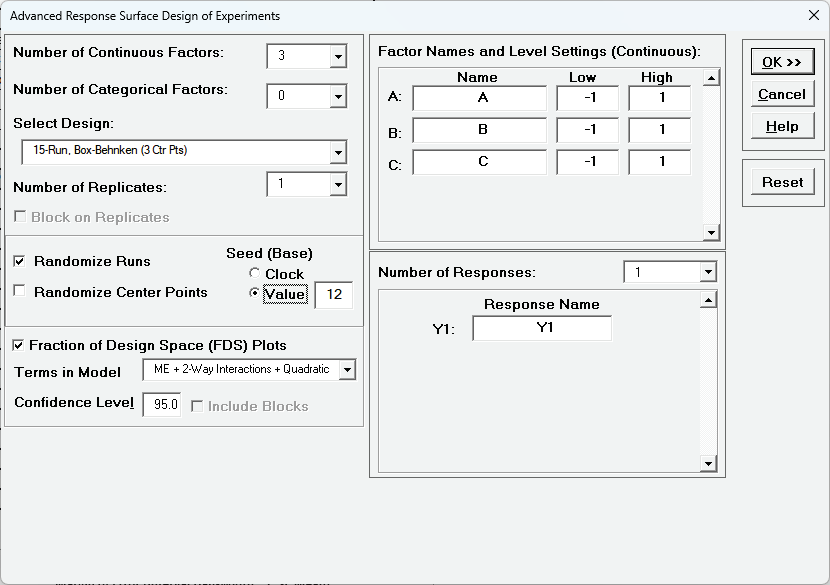
26. This is a 3 Factor, 15 Run, Box-Behnken Design with 3 Center Points and 1 Replicate. Click OK.





27. To create Overly FDS Plots, click SigmaXL > Design of Experiments > Advanced Design of Experiments: Overlay FDS Plots. Select >FDS Plot Sheets and enter Legend names as shown:







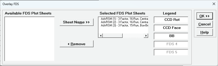
28. Click OK.







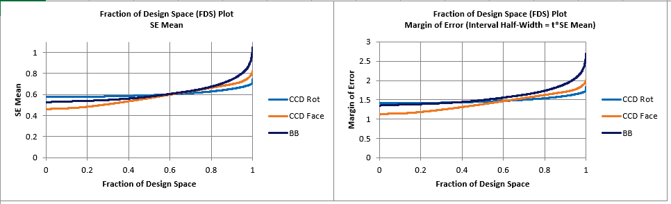
CCD Rotatable (CCD Rot) has the flattest FDS Plot, and the smallest SE Mean and Margin of Error in 40% of the design space. This design is recommended if five levels are possible.




CCD Face Centered (CCD Face) has the smallest SE Mean and Margin of Error in 60% of the design space.




Box-Behnken (BB) has the largest SE Mean and Margin of Error in 40% of the design space. This is due to not having points at the cube corners.




Summary: Interpreting the FDS Plot

• You can use FDS Plots to compare and select number of replicates, number of center points, Central Composite alpha axial value, Central Composite vs Box-Behnken and optimality criterion.
• SE Mean and Margin of Error - smaller is better, flatter is better, over the majority of the design space.
• Try to achieve this with minimum runs.
• If the process standard deviation is known, multiply the SE Mean and Margin of Error by the standard deviation to estimate the actual prediction error vs fraction of design space.