Example 1: Design and Analysis of Catapult Full Factorial
Experimentusing Advanced Design of Experiments
To demonstrate some of the features in Advanced Design of Experiments, we will revisit the example given in Part C – Design and Analysis of Catapult Full Factorial Experiment. In particular, we will focus on the Design Power Information and the Cube Plot.
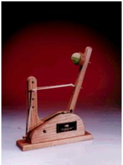
Catapults are frequently used in Six-Sigma or Design of Experiments training. They are a powerful teaching tool and make the learning fun. The response variable (Y) is distance, with the goal being to consistently hit a target of 100 inches.Using process knowledge, we will limit ourselves to 3 factors: Pull Back Angle, Stop Pin and Pin Height. Pull Back will be varied from 160 to 180 degrees, Stop Pin will be positions 2 and 3 (count from the back), and Pin Height will be positions 2 and 3 (count from the bottom).
-
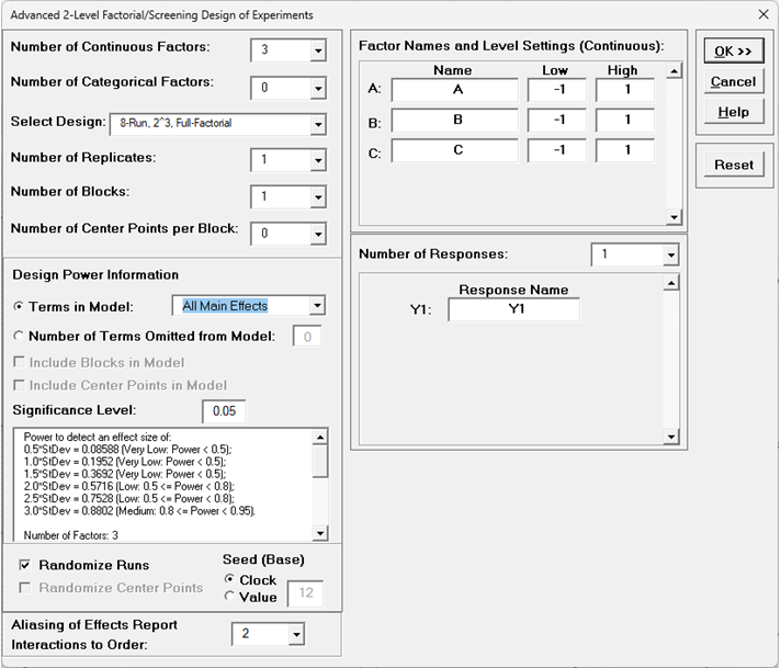
Click SigmaXL > Design of Experiments > Advanced Design of Experiments: 2-Level Factorial/Screening > 2-Level Factorial/Screening Designs.
Select Number of Continuous Factors = 3, Number of Categorical Factors = 0. Select Design as 8-Run, 2^3 Full-Factorial, Number of Replicates = 1.
-
With the default Design Power InformationTerms in Model=All Main Effects, you can scroll to view the power report as shown:
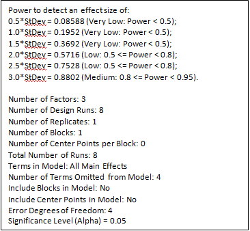
With a Main Effects model, this design has very low power (< 0.5) to detect an effect size of 1.0*StDev, low power (0.5 to < 0.8) to detect an effect size = 2.0*StDev and medium power
(0.8 to < 0.95) to detect an effect size = 3.0*StDev. The error degrees of freedom for the power calculation= 4 come from the 3 two-way interaction terms and 1 three-way interaction term that are removed from the model. Note that this power analysis differs from that shown in Part C – Design and Analysis of Catapult Full Factorial Experiment, where all terms are removed from the model but 3 center points are assumed in order to estimate power.
-
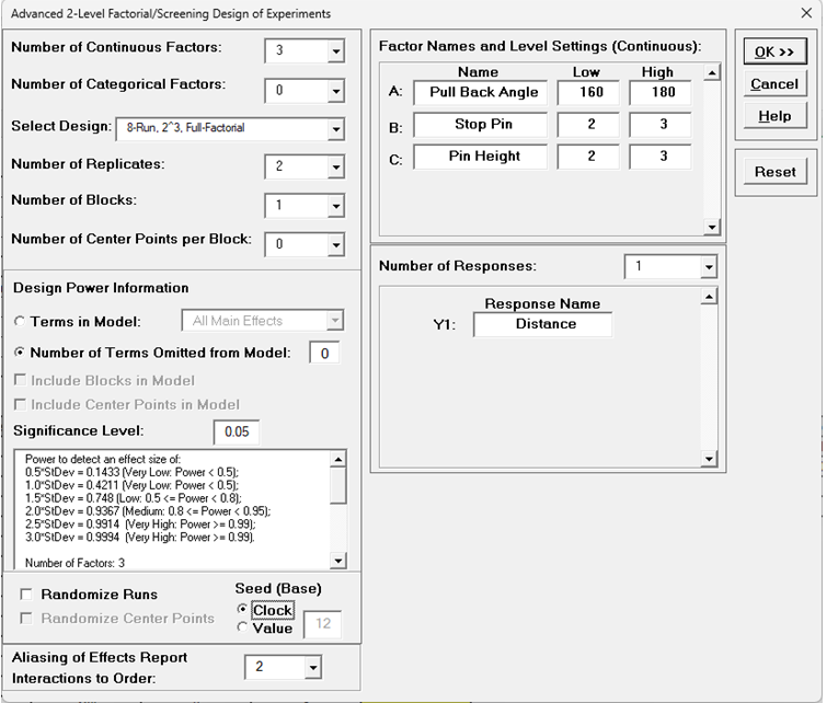
Now select Number of Replicates= 2 to match the earlier design. Enter Factor Names and Level Settings as shown. Uncheck Randomize Runs. This will display the design in standard order.
If this experiment is being carried out with a physical catapult, the runs should be performed in random order.
-
For Design Power Information select Number of Terms Omitted from Model = 0. This specifies that all main effects, two-way interactions and the three-way interaction are included in the model
for power calculation. The error degrees of freedom will come from the replicates. You can scroll to view the power report as shown:
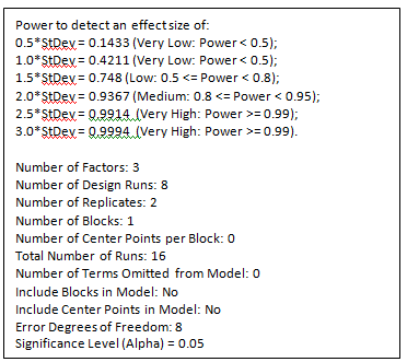
This design has very low power (< 0.5) to detect an effect size of 1.0*StDev, medium power (0.8 to < 0.95) to detect an effect size = 2.0*StDev and very high power (> 0.99) to detect an effect size = 3.0*StDev. This is a dramatic improvement over the single replicate case. This power analysis matches that shown in Part C – Design and Analysis of Catapult Full Factorial Experiment, but provides more detailed information such as the exact power values and the error degrees of freedom.
-
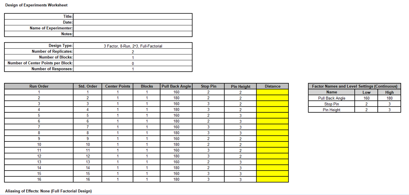
Click OK. The following Design of Experiments Worksheet is produced including the Factor Names and Level Settings summary, and Design Power Information. There is no Aliasing of Effects report since this is a full-factorial design:
-
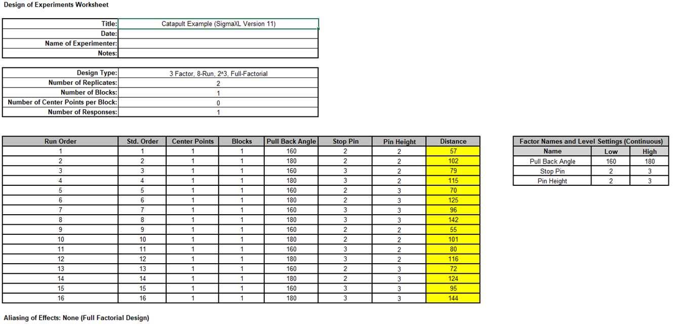
Open the file Catapult DOE V11.xlsx. This has the design worksheet populated with Catapult Distance values.
-
Click SigmaXL > Design of Experiments > Advanced Design of Experiments: 2-Level Factorial/Screening > Analyze 2-Level Factorial/Screening Design.For comparison to the earlier analysis see Analysis of Catapult Full Factorial Experiment with Advanced Multiple Regression.
-
Select Responses and Model Terms as shown with Term Generator as ME+2-Way Interactions. Check Residual Plots, Main Effects Plots,
Interaction Plots and Cube Plots. We will use the defaults for Advanced Options and leave Box-Cox Transformation unchecked.
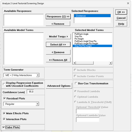
Cube Plots are available for 2-Level Factorial/Screening designs when there are 2 to 5 factors. Cube Plots show Response Fitted Means in each cube corner. If there are center points in the model, the fitted values for center points are also shown. If there are blocks in the model, then Averaging Over Blocks is used. If there are 2 Factors, then a Square Plot is produced. If there are 4 Factors, then two Cube Plots are given. If there are 5 Factors, then four cube plots are produced.
Note that there is no option to standardize/code continuous predictors or option for coding categorical predictors. Continuous predictors are always coded as Factor high/low = +1/-1, which is slightly different than the Advanced Multiple Regression option Xmax = +1, Xmin = -1. In Analyze DOE, if the worksheet minimum or maximum has been modified by the user, those changes do not affect the determination of coded +1/-1. In Advanced Multiple Regression the modified maximum value would be coded as +1 or the modified minimum value would be coded as -1.
Categorical predictors are coded as (-1/0/+1).
Test/Withhold Sample is not available for DOE Analysis.
-
Click Advanced Options.

The Advanced Options for Analyze DOE are similar to those in Advanced Multiple Regression. The Box-Tidwell Test and Power Transformation Recommendation for Continuous Predictors option is not available since the automatic coding produces 0 and -1 factor values which cannot be transformed.
-
We will use the default options. Click OK.
-
Click OK. The DOE Multiple Regression report for Distance is given:
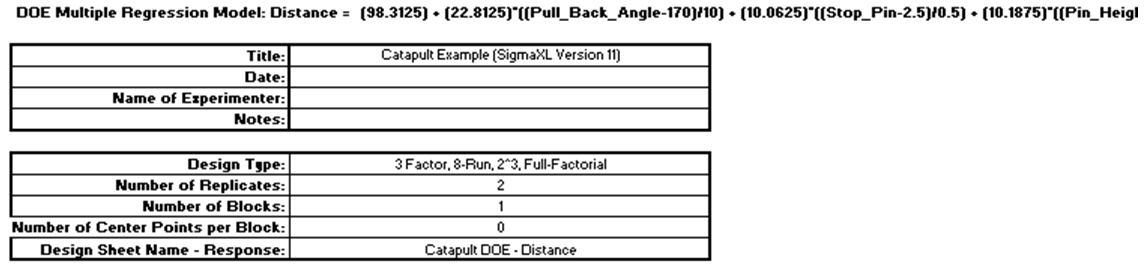
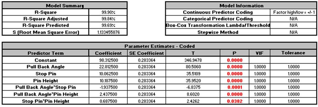
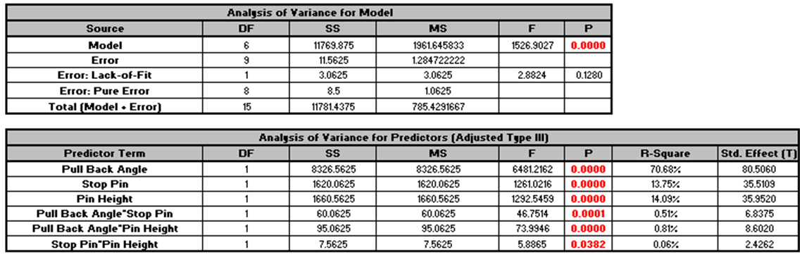
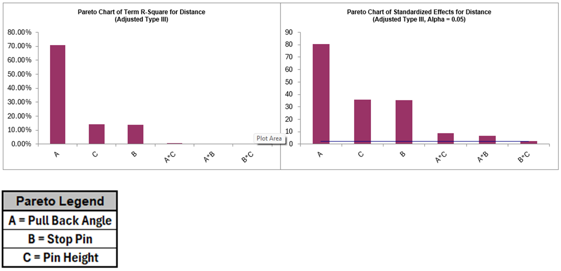
The DOE Multiple Regression report shows that all factors are significant with Pull Back Angle being the dominant factor affecting the distance response. These results are very similar to the earlier Advanced Multiple Regression analysis, except for the Continuous Predictor Coding = Factor high/low = +1/-1 as discussed above. Also, the Pareto Legend uses the factor letters A, B, C whereas the Pareto Legend for Advanced Multiple Regression uses X1, X2, X3.
Click on the Residuals sheet to view the Residual Plots. They are the same as those in the previous analysis and look very good, approximately normal, with no obvious patterns.
The Main Effects and Interaction Plots are also the same, so they will not be discussed further here.
-
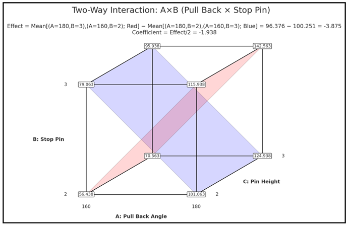
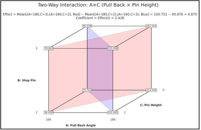
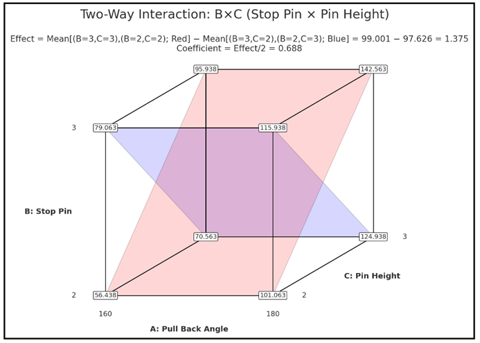
Click on the CubePlot sheet to view the Cube Plot:
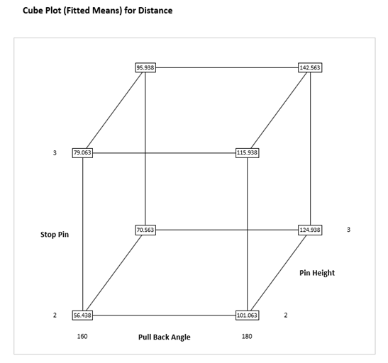
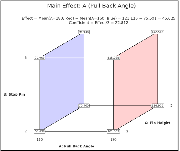
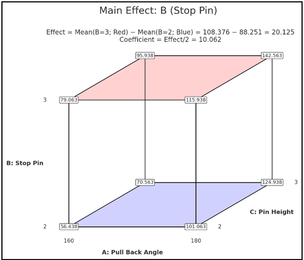
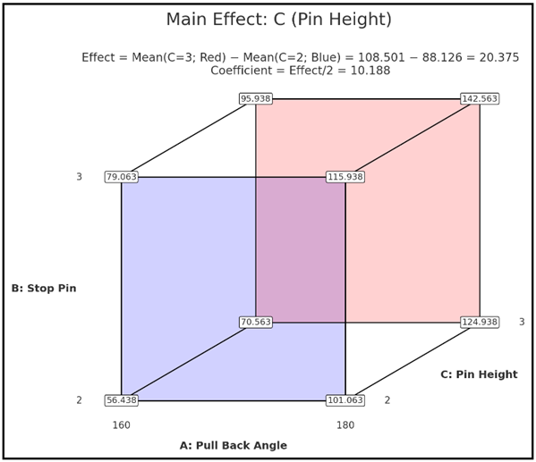
We can see from the Cube Plot that our target distance = 100 occurs approximately with Pull Back Angle = 180, Stop Pin = 2 and Pin Height = 2. The Cube Plot can be used to obtain a geometric representation of the Main Effects and Two-Way Interaction Effects as shown. The Coefficient values(= Effect/2) match those given in the Parameter Estimates table above.
-
The steps for optimization were given in the previous analysis using the Predicted Response Calculator and Optimization. We will not review that again here.


