ARIMA – Multiple Seasonal Decomposition (MSD) Forecast

Open Monthly Airline Passengers - Series G.xlsx (Sheet 1 tab). This is the Series G data from Box and Jenkins, monthly total international airline passengers for January 1949 to December 1960. See the Run Chart, ACF/PACF Plots, Spectral Density Plot and Seasonal Trend Decomposition Plots for this data. The Multiple Seasonal Decomposition (MSD) option is not necessary for this data, but by way of introduction, we will use this to compare to the previous ARIMA analysis.
Click SigmaXL > Time Series Forecasting > ARIMA Forecast > Multiple Seasonal Decomposition Forecast. Ensure that the entire data table is selected. If not, check Use Entire Data Table. Click Next.
Select Monthly Airline Passengers, click Numeric Time Series Data (Y) >>. Select Date, click Optional Time Axis Labels >>. Check Display ACF/PACF/LB Plots and Display Residual Plots. Check Specify Model Periods. Set Withhold Periods = 24. Select Withhold Forecast Type: Multi-Step-Ahead with Prediction Interval at Start of Withhold. Select Seasonal Frequency Specify and enter 12. Check Box-Cox Transformation and select Rounded Lambda. We will use the default Prediction Interval = 95.0 %.

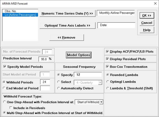
• Seasonal Frequency can have multiple entries however, we recommend no more than 3 values.
Click Model Options.
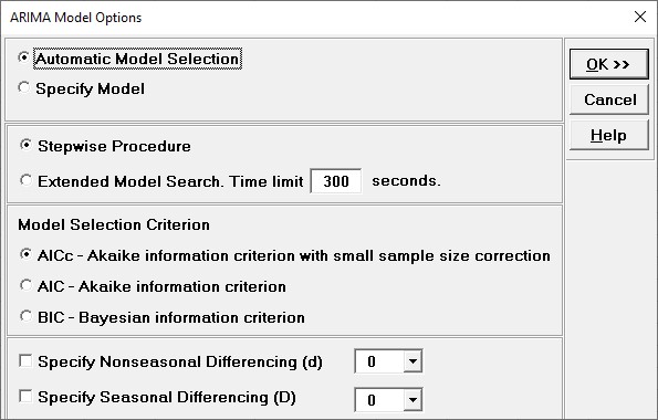
We will use the default Automatic Model Selection with AICc as the Model Selection Criterion. Click OK to return to the ARIMA MSD Forecast dialog. Click OK. The ARIMA forecast report is given:
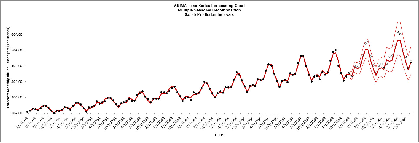
Scroll down to view the ARIMA Model header:
The ARIMA Model Summary is given as:

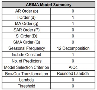
This is a summary of the model information for the deseasonalized data: ARIMA (0,1,1) with a constant. Seasonal Frequency = 12 using Decomposition and Model Selection Criterion = “AICc”. There are no seasonal terms in the model. The Box-Cox Transformation is “Rounded Lambda” with Lambda = 0 (Ln transformation).
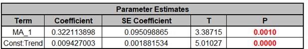
The Parameter Estimates for the deseasonalized Airline Passenger data are:
The ARIMA Model Statistics are:

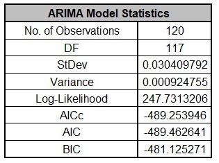
• The number of observations, n = 144 – 24 (withhold) = 120

• Degrees of freedom (DF) = 120 (n) – 3 (2 terms in the model, 1 nonseasonal difference) = 117

• Note that the model statistics are based on the Ln transformed data, not the original data.

• Comparing to the Exponential Smoothing MSD Model Statistics, we see that the StDev and Variance are approximately equal, but the Log-Likelihood, AICc, AIC and BIC are very different. This is due to different formulas being used in the Likelihood function. You cannot use Information Criteria to compare ARIMA and Exponential Smooth models to determine which model has the best fit.
The Forecast Accuracy metrics are:

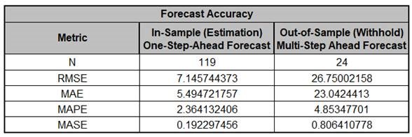
Comparing to Exponential Smoothing MSD Forecast Accuracy metrics, we see that the ARIMA MSD results are approximately the same.

Forecast Accuracy metrics are calculated using the actual raw data versus inverse transformed forecast as displayed in the Forecast Chart and Table, so allow comparison across all model types and transformations.
Click on the ARIMA MSD ACF PACF LB sheet to view the ACF/PACF/LB Plots:

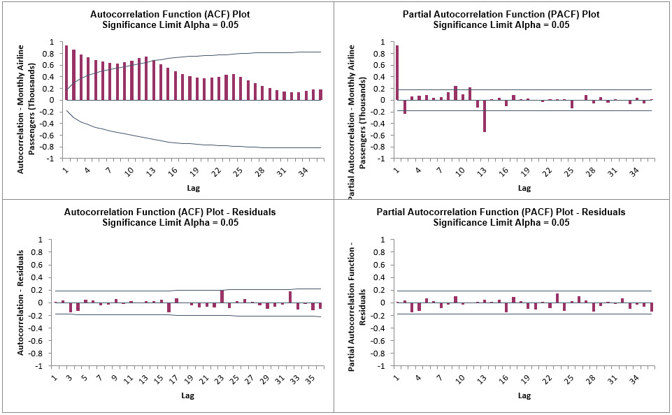
The ARIMA MSD ACF/PACF Residuals Plots are similar to the Exponential Smoothing MSD ACF/PACF/LB Plots and indicate that the autocorrelation has been accounted for in the model. All of the Ljung-Box P-Values are blue (i.e., not significant), with P-Values > .05.
Click on the ARIMA MSD Residuals sheet to view the Residual Plots:

The residuals are approximately normally distributed, with a roughly straight line on the normal probability plot. There are no obvious extreme outliers or patterns in the charts. The residual plots are approximately the same as those given previously in Exponential Smoothing MSD Residual Plots.

Since a Box-Cox transformation was used, the residuals are in Ln transformed units.
Open Half-Hourly Multiple Seasonal Electricity Demand - Taylor.xlsx (Sheet 1 tab). This is half-hourly electricity demand (MW) in England and Wales from Monday, June 5, 2000 to Sunday, August 27, 2000 (taylor, R forecast). This data has multiple seasonality with frequency = 48 (observations per day) and 336 (observations per week), with a total of 4032 observations. See the Run Chart, ACF/PACF Plots, Spectral Density Plot and Seasonal Trend Decomposition Plots for this data.
Click SigmaXL > Time Series Forecasting > ARIMA Forecast > Multiple Seasonal Decomposition Forecast. Ensure that the entire data table is selected. If not, check Use Entire Data Table. Click Next.
Select Demand, click Numeric Time Series Data (Y) >>. Check Display ACF/PACF/LB Plots and Display Residual Plots. Check Specify Model Periods. Set Withhold Periods = 96. Select Withhold Forecast Type: Multi-Step-Ahead with Prediction Interval at Start of Withhold. Check Seasonal Frequency with Specify = 48 336. Leave Box-Cox Transformation unchecked. We will use the default Prediction Interval = 95.0 %.

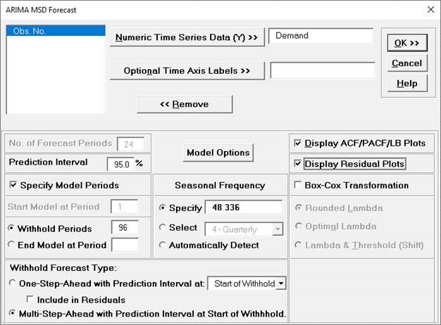
Withhold Periods is 2*dominant seasonal frequency (48). Dominant frequency is obtained from the Spectral Density Plot. Start Model at Period = 1 is always greyed out for MSD.
Click Model Options.
We will use the default Automatic Model Selection with AICc as the Model Selection Criterion. Click OK to return to the ARIMA MSD Forecast dialog. Click OK. The ARIMA forecast report is given:
We will want to zoom in on the last 3 days, i.e., 144 half-hourly time periods, using chart scrolling. Click SigmaXL Chart Tools > Enable Scrolling

You may be prompted with a warning message that custom formatting on the chart will be cleared. You can avoid seeing this warning by checking Save this choice as default and do not show this form again.
Click OK. The scroll dialog appears allowing you to specify the Start Period and Window Width. Enter Start Period = 3888 and Window Width = 144:

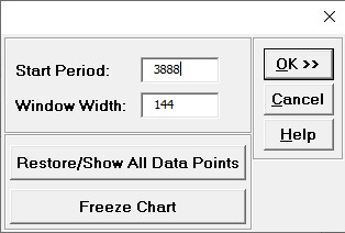
At any point, you can click Restore/Show All Data Points or Freeze Chart. Freezing the chart will remove the scroll and unload the dialog. The scroll dialog will also unload if you change worksheets. To restore the dialog, click SigmaXL Chart Tools > Enable Scrolling.
Click OK. A scroll bar appears beneath the forecast chart. You can also change the Start Subgroup and Window Width and Update.

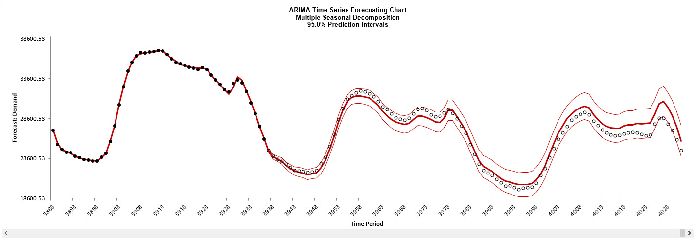
You can scroll through by clicking to the right or left, with the specified window width of 144.

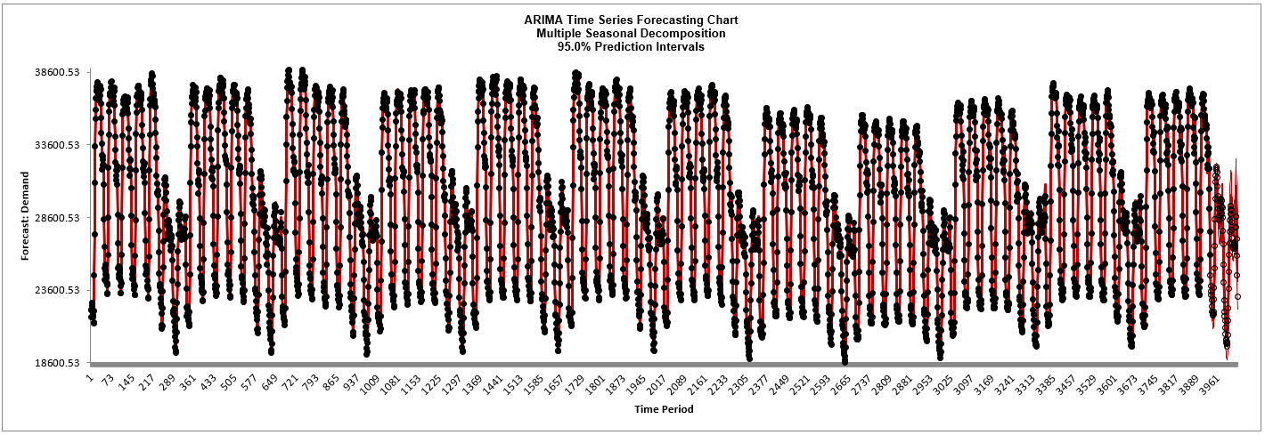
The blank dots are the data values in the withhold sample with a multi-step forecast and prediction intervals displayed at the start of the withhold sample. The model does quite well at predicting the withhold 96 half-hour demand values. Note that the prediction error increases the further out we predict. The ARIMA MSD Forecast Chart looks approximately the same as the previous Exponential Smoothing MSD Forecast Chart.

Click Cancel to exit the scroll dialog.
Scroll down to view the ARIMA Model header:
The ARIMA Model Summary is given as:

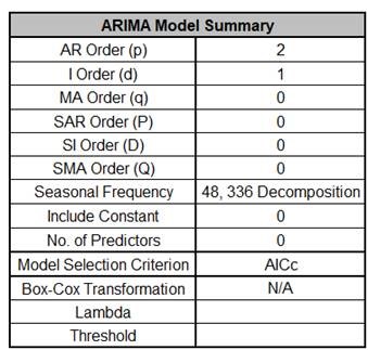
This is a summary of the model information for the deseasonalized data: ARIMA (2,1,0) without a constant. Seasonal Frequency = 48, 336 using Decomposition and Model Selection Criterion = “AICc”. There are no seasonal terms in the model.
The Parameter Estimates for the deseasonalized Demand data are:

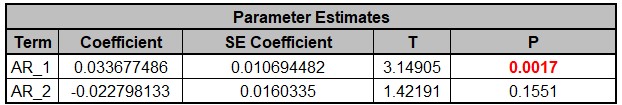
ARIMA Parameter Estimates include significance tests; P-Values < .05 are significant and highlighted in red. This may be useful for model refinement with multiple predictors but for AR/MA model order selection, minimum AICc should be used, rather than significance tests (see Kostenko, A.V. and Hyndman, R.J. ).
The ARIMA Model Statistics are:

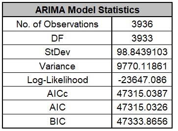
• The number of observations, n = 4032 – 96 (withhold) = 3936

• Degrees of freedom (DF) = 3936 (n) – 3 (2 terms in the model, 1 nonseasonal difference) = 3933

• Note that the model statistics are calculated using the deseasonalized data.
The Forecast Accuracy metrics are:

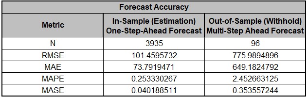
As expected, the Out-of Sample (Withhold) Multi-Step-Ahead Forecast errors are larger than the In-Sample (Estimation) One-Step-Ahead Forecast errors. Note, if we were primarily interested in a short term one-step ahead forecast, then we would have selected Withhold Forecast Type: One-Step-Ahead and the above table would show Out-of-Sample (Withhold) One-Step-Ahead Forecast errors.

Comparing to the previous Exponential Smoothing MSD Forecast Accuracy metrics, we see that the ARIMA MSD results are approximately the same.

Forecast Accuracy metrics are calculated using the actual raw data versus forecast as displayed in the Forecast Chart and Table so, unlike the model statistics above, allows comparison across all forecast model types and transformations.
The Forecast Table is given as:

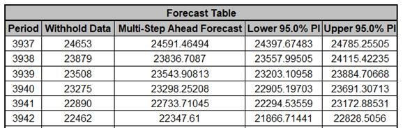
These are the same forecast and prediction interval values displayed in the Forecast Chart, but provided for further analysis or charting (e.g., a run chart of the forecast errors). The Withhold Data is also displayed.
Click on the ARIMA MSD ACF PACF LB sheet to view the ACF/PACF/LB Plots:

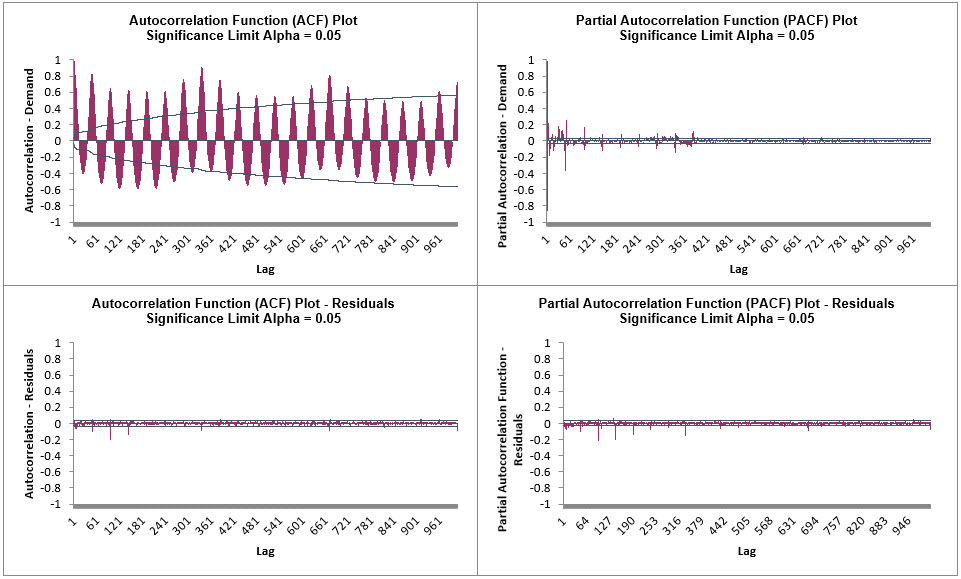
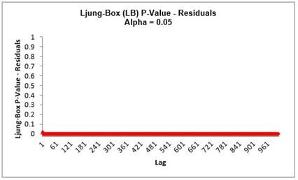
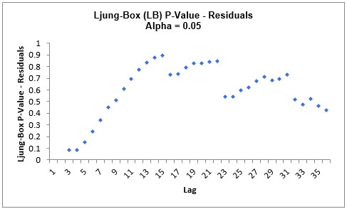
The ACF/PACF Residuals Plots indicate that much of the autocorrelation has been accounted for in the model, but the Ljung-Box plot shows that some significant autocorrelation still remains (the red P-Values are significant at alpha=.05) - so the model can potentially be improved. This does not mean that the model is a bad model, it can still be very useful for prediction purposes, but the prediction intervals may not provide accurate coverage.
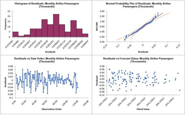
Click on the ARIMA MSD Residuals sheet to view the Residual Plots:

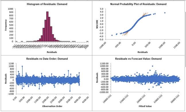
Similar to the Exponential Smoothing MSD Residual Plots, the residuals are not normally distributed and there are extreme outliers. These should be investigated with a control chart on the residuals. Outliers in Electricity Demand are often explained by Temperature.

ARIMA does not have a theoretical frequency limit, but for computational efficiency and to minimize the potential loss of observations through differencing, we recommend using ARIMA – Multiple Seasonal Decomposition (MSD) for seasonal frequency greater than 52 (or with multiple frequencies).

The seasonal component is first removed through decomposition, a nonseasonal ARIMA model fitted to the remainder (+trend), and then the seasonal component is added back in. For forecasting, a naïve seasonal forecast is used on the seasonal component. Note that the prediction intervals are derived from the ARIMA model and do not include uncertainty in the seasonal component.

As the name implies, Multiple Seasonal Decomposition (MSD) also accommodates multiple seasonality, for example the half-hourly data with a seasonal frequency of 48 observations per day and 336 observations per week. When using MSD, it is recommended to limit the forecast period to 2*dominant seasonal frequency.