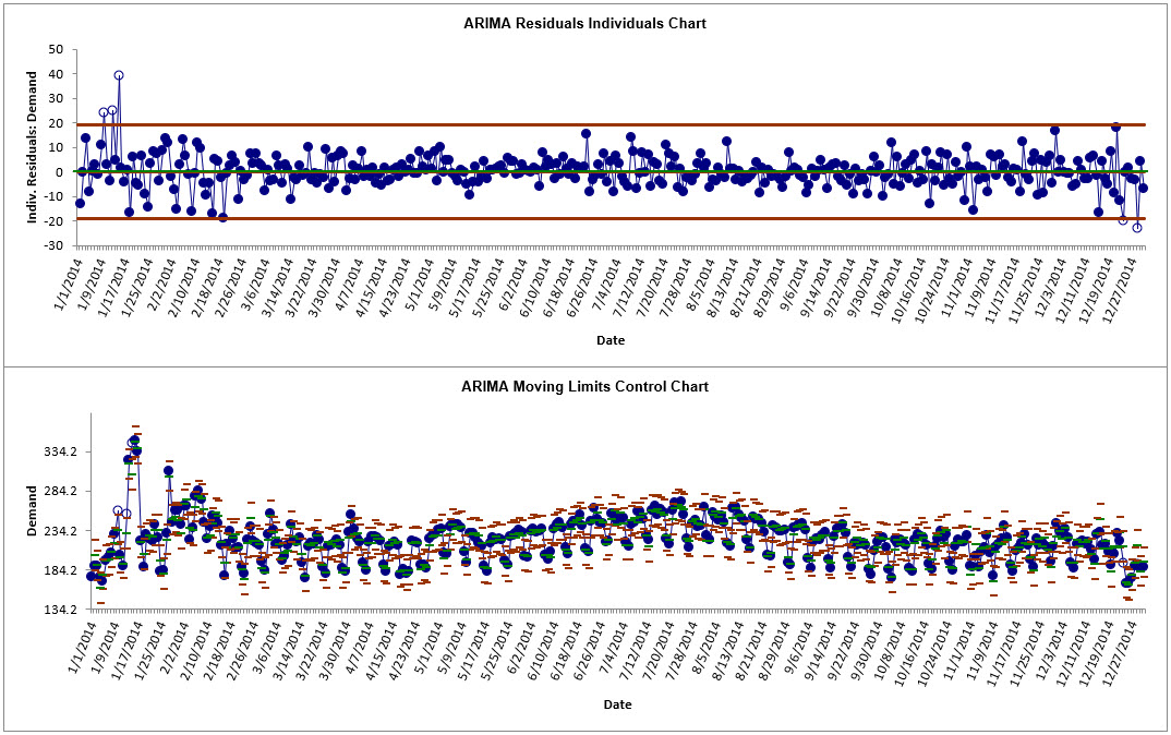
An Individuals control chart is created
using the residuals of the ARIMA with Predictors forecast model.
The ARIMA with Predictors model supports continuous or categorical
predictors. See ARIMA Forecast with Predictors for more information.
The Moving Limits chart uses the one step prediction as the
center line, so the control limits will move with the center line.
If a Box-Cox transformation is used then an inverse transformation
is applied to calculate the control limits.
The
popular Show Last 30 and Scroll features in SigmaXL Chart Tools
are available for these control charts. Currently, the Add Data
feature is not supported in ARIMA Control Chart with Predictors.
Note that a Moving
Range Chart and Tests for Special Causes are not available here, but the user can store and
select Residuals, then create with SigmaXL > Control Charts > Individuals
& Moving Range.
Open Daily Electricity Demand with Predictors
ElecDaily.xlsx (Sheet 1 tab). This is
daily electricity demand (GW) for the state of Victoria,
Australia, every day during 2014. Temp (C) is the maximum daily
temperature in degrees Celsius for the city of Melbourne. TempSq
is Temperature squared. WorkDay takes on the value 1 on work
days and 0 otherwise. This data has a seasonal frequency = 7
(observations per week). See the Run Chart, ACF/PACF Plots,
Spectral.html and Seasonal Trend Decomposition Plots for
this data.
Click
SigmaXL > Time Series Forecasting > ARIMA Control Chart > Control
Chart
with Predictors. Ensure that the entire data table is selected. If not,
Use Entire Data Table. Click Next.
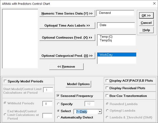
Select Demand, click Numeric Time Series Data
(Y) >>; select Date, click Optional X-Axis
Labels >>; select Temp (C) and TempSq,
click Optional Continuous Pred. >>; select
WorkDay, click Optional Categorical Pred. >>.
Uncheck Display ACF/PACF/LB Plots and
Display Residual Plots. Check Seasonal
Frequency with Select = 7 - Daily (or
Specify = 7). Leave Specify Model
Periods and Box-Cox Transformation
unchecked.
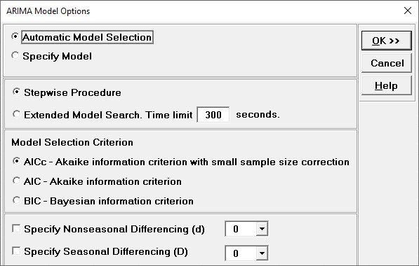
Click Model Options.
Select Automatic Model Selection. We will use
the defaults: Stepwise Procedure and
Model Selection Criterion: AICc Akaike information criterion
with small sample size correction, leave
Specify Nonseasonal Differencing (d) and
Specify Seasonal Differencing (D) unchecked.
Click OK to return to
the ARIMA with Predictors Control Chart dialog. Click OK.
This is a complex model, so computation time will be
approximately one to two minutes. The ARIMA with Predictors
control charts are produced:
Scroll down to view the ARIMA Model
header:
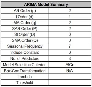
The ARIMA Model Summary is given as:
This is a summary of the model information: ARIMA (2,1,2) (2,0,0) with no constant
and 3 predictors. Seasonal Frequency = 7; Model Selection Criterion = AICc and
Box-Cox Transformation = N/A because Box-Cox Transformation was unchecked.