How Do I Create a Capability Combination Report for Non-Normal Data?

Capability Combination Report (Individuals Nonnormal)

An important assumption for process capability analysis is that the data be normally distributed. The Capability Combination Report (Individuals Nonnormal) allows you to transform the data to normality or utilize nonnormal distributions, including:

• Box-Cox Transformation (includes an automatic threshold option so that data with negative values can be transformed)
• Johnson Transformation
• Distributions supported:
• Half-Normal
• Lognormal (2 & 3 parameter)
• Exponential (1 & 2 parameter)
• Weibull (2 & 3 parameter)
• Beta (2 & 4 parameter)
• Gamma (2 & 3 parameter)
• Logistic
• Loglogistic (2 & 3 parameter)
• Largest Extreme Value
• Smallest Extreme Value
• Automatic Best Fit based on AD p-value

For technical details, see Appendix: Statistical Details for Nonnormal Distributions and Transformations. Also see Andrew Sleeper, Six Sigma Distribution Modeling, for further information on these methods.

Note that these transformations and distributions are particularly effective for inherently skewed data but should not be used with bimodal data or where the nonnormality is due to outliers (typically identified with a Normal Probability Plot). In these cases, you should identify the reason for the bimodality or outliers and take corrective action. Another common reason for nonnormal data is poor measurement discrimination leading to “chunky” data. In this case, attempts should be made to improve the measurement system.

Box-Cox Transformation

SigmaXL’s default setting is to use the Box-Cox transformation which is the most common approach to dealing with nonnormal data. Box-Cox is used to convert nonnormal data to normal by applying a power transformation, Y^lambda, where lambda varies from -5 to +5. You may select rounded or optimal lambda. Rounded is typically preferred since it will result in a more “intuitive” transformation such as Ln(Y) (lambda=0) or SQRT(Y) (lambda=0.5). If the data includes zero or negative values, select Lambda & Threshold. SigmaXL will solve for an optimal threshold which is a shift factor on the data so that all of the values are positive.

1. Open the file Nonnormal Cycle Time2.xls. This contains continuous data of process cycle times. The Critical Customer Requirement is: USL = 1000 minutes.
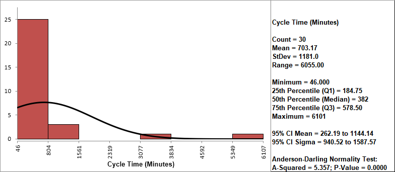
2. Let’s begin with a view of the data using Histograms and Descriptive Statistics. Click SigmaXL > Graphical Tools > Histograms & Descriptive Statistics.
3. Ensure that entire data table is selected. If not, check Use Entire Data Table. Click Next.
4. Select Cycle Time (Minutes), click Numeric Data Variable (Y) >>. Click OK.

Clearly this is a process in need of improvement. To start, we would like to get a baseline process capability. The problem with using regular Capability analysis is that the results will be incorrect due to the nonnormality in the data. The Histogram and AD p-value < .05 clearly show that this data is not normal.

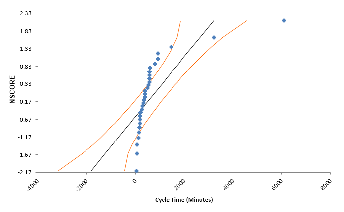
5. We will confirm the nonnormality by using a Normal Probability Plot. Click Sheet 1 Tab (or F4). Click SigmaXL > Graphical Tools > Normal Probability Plots.
6. Ensure that the entire data table is selected. If not, check Use Entire Data Table. Click Next.
7. Select Cycle Time (Minutes), click Numeric Data Variable (Y) >>. Click OK. A Normal Probability Plot of Cycle Time data is produced:



8. The curvature in this normal probability plot confirms that this data is not normal.
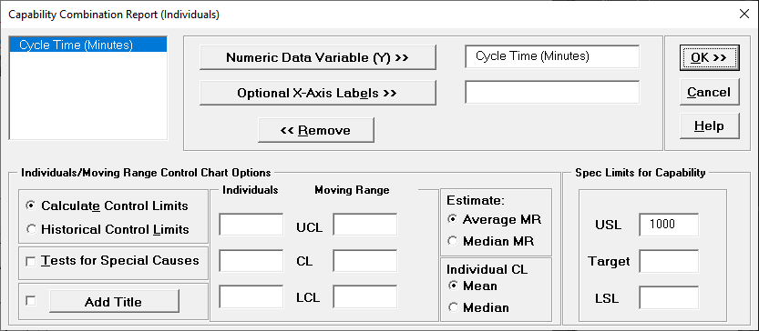
9. For now, let us ignore the nonnormal issue and perform a Process Capability study assuming a normal distribution. Click Sheet 1 Tab. Click SigmaXL > Process Capability > Capability Combination Report (Individuals).
10. Select Cycle Time (Minutes), click Numeric Data Variable (Y) >>. Enter USL = 1000; delete previous Target and LSL settings.
    
    


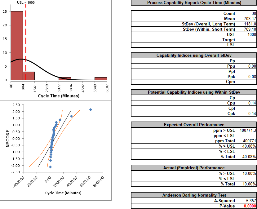
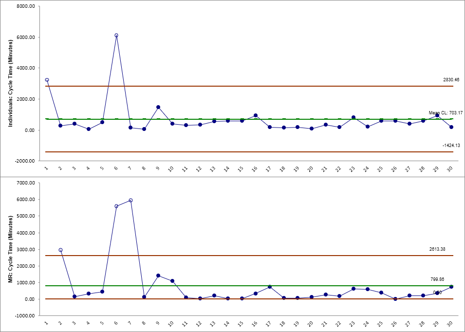
11. Click OK. The resulting Process Capability Report is shown below:

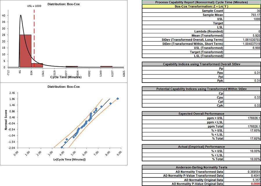
Notice the discrepancy between the Expected Overall (Theoretical) Performance and Actual (Empirical) Performance. This is largely due to the nonnormality in the data, since the expected performance assumes that the data is normal. So why not just use the actual performance and disregard the expected? This would not be reliable because the sample size, n = 30, is too small to estimate performance using pass/fail (discrete) criteria.

Also note that the process appears to be out-of-control on both the individuals and moving range charts.

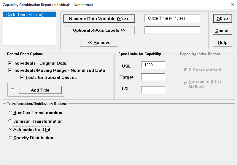
12. We will now perform a process capability analysis using the Capability Combination Report for Nonnormal Individuals. Click Sheet 1 Tab (or F4). Click SigmaXL > Process Capability > Nonnormal > Capability Combination Report (Individuals Nonnormal). Ensure that the entire data table is selected. If not, check Use Entire Data Table. Click Next.
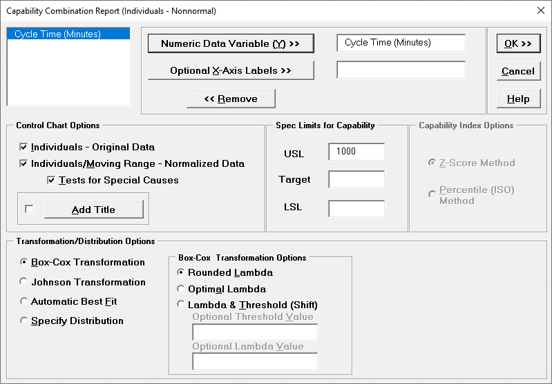
13. Select Cycle Time (Minutes), click Numeric Data Variable (Y) >>. Enter USL = 1000. We will use the default selection for Transformation/Distribution Options: Box-Cox Transformation with Rounded Lambda. Check Tests for Special Causes as shown:




14. Click OK. The resulting Process Capability Combination report is shown below:

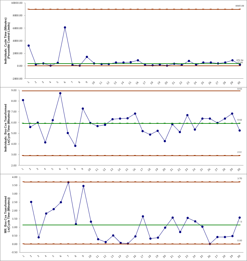
The AD Normality P-Value Transformed Data value of 0.404 confirms that the Box-Cox transformation to normality was successful. The process capability indices and expected performance can now be used to establish a baseline performance. Note that there are no out-of-control signals on the control charts, so the signals observed earlier when normality was assumed were false alarms.

The Individuals – Original Data chart displays the untransformed data with control limits calculated as:
UCL = 99.865 percentile
CL = 50th percentile
LCL = 0.135 percentile

The benefit of displaying this chart is that one can observe the original untransformed data. Since the control limits are based on percentiles, this represents the overall, long term variation rather than the typical short term variation. The limits will likely be nonsymmetrical.

The Individuals/Moving Range – Normalized Data chart displays the transformed z-values with control limits calculated using the standard Shewhart formulas for Individuals and Moving Range charts. The benefit of using this chart is that tests for special causes can be applied and the control limits are based on short term variation. The disadvantage is that one is observing transformed data on the chart rather than the original data.

Automatic Best Fit

Now we will redo the capability analysis using the Automatic Best Fit option.

15. Click Recall SigmaXL Dialog menu or press F3 to recall last dialog. Select Automatic Best Fit as shown:




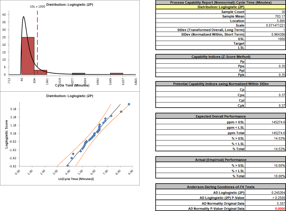
16. Click OK. The resulting Process Capability Combination report is shown below. Please note that due to the extensive computations required, this could take up to 1 minute (or longer for large datasets):

The 2 Parameter Loglogistic distribution was selected as the best fit distribution. For details on how this selection was made, see Appendix: Statistical Details for Nonnormal Distributions and Transformations.

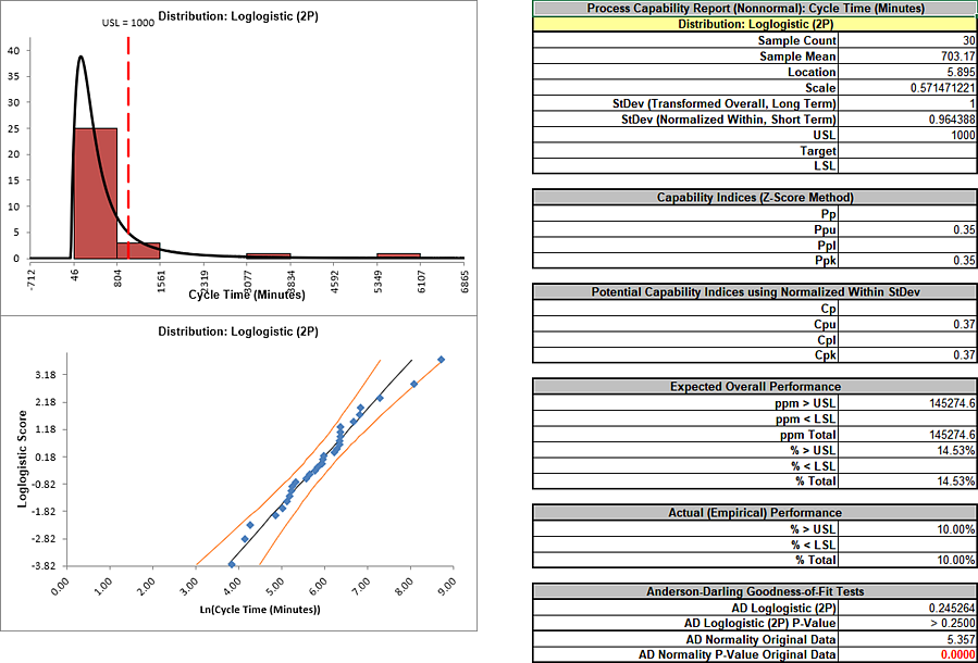
The Anderson Darling statistic for the Loglogistic distribution is 0.245 which is less than the 0.37 value for the AD Normality test of the Box-Cox transformation indicating a better fit. (Note that published AD p-values for this distribution are limited to a maximum value of 0.25. The best fit selection uses a p-value estimate that is obtained by transforming the data to normality and then using a modified Anderson Darling Normality test on the transformed data).

Distribution Fitting

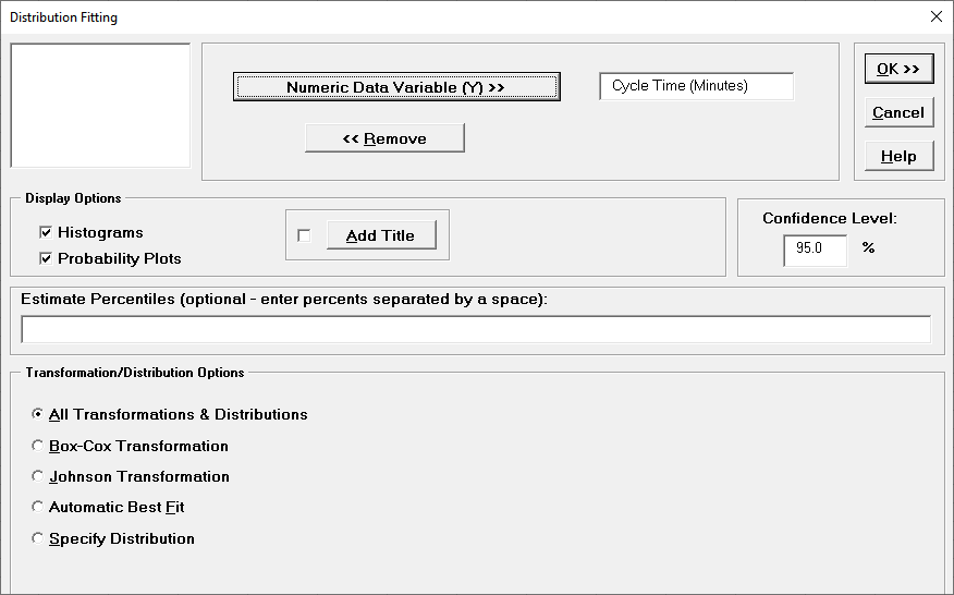
Another helpful tool to evaluate transformations and distributions is Distribution Fitting.

17. Click Sheet 1 Tab (or F4). Click SigmaXL > Process Capability > Nonnormal > Distribution Fitting. Ensure that the entire data table is selected. If not, check Use Entire Data Table. Click Next.
18. Select Cycle Time (Minutes), click Numeric Data Variable (Y) >>. We will use the default selection for Transformation/Distribution Options: All Transformations & Distributions as shown:




19. Click OK. The resulting Distribution Fitting report is shown below. Please note that due to the extensive computations required, this could take up to 1 minute (or longer for large datasets):

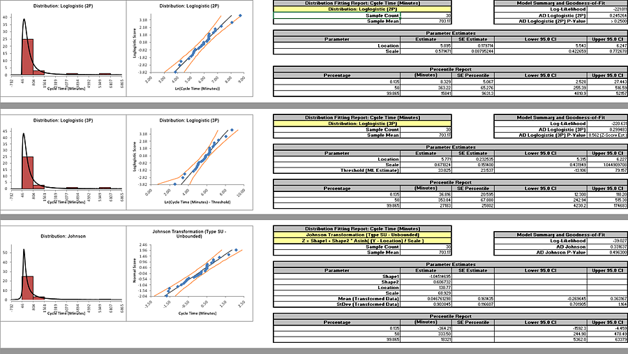
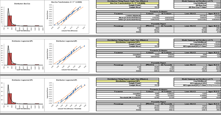
The distributions and transformations are sorted in descending order using the AD Normality p-value on the transformed z-score values. Note that the first distribution shown may not be the selected “best fit”, because the best fit procedure also looks for models that are close but with fewer parameters.

The reported AD p-values are those derived from the particular distribution. The AD p-value is not available for distributions with a threshold (except Weibull), so the AD Normality p-value on the transformed z-score values is used (labeled as Z-Score Est.).

Since the sort order is based on the AD p-values from Z-Score estimates, it is possible that the reported distribution based AD p-values may not be in perfect descending order. However any discrepancies based on sort order will likely not be statistically or practically significant.

Some data will have distributions and transformations where the parameters cannot be solved (e.g., 2-parameter Weibull with negative values). These are excluded from the Distribution Fitting report.

The parameter estimates and percentile report includes a confidence interval as specified in the Distribution Fitting dialog, with 95% being the default. Note that the wide intervals here are due to the small sample size, n = 30.

The control limits for the percentile based Individuals chart will be the 0.135% (lower control limit), 50% (center line, median) and 99.865% (upper control limit). Additional percentiles may be entered in the Distribution Fitting dialog.

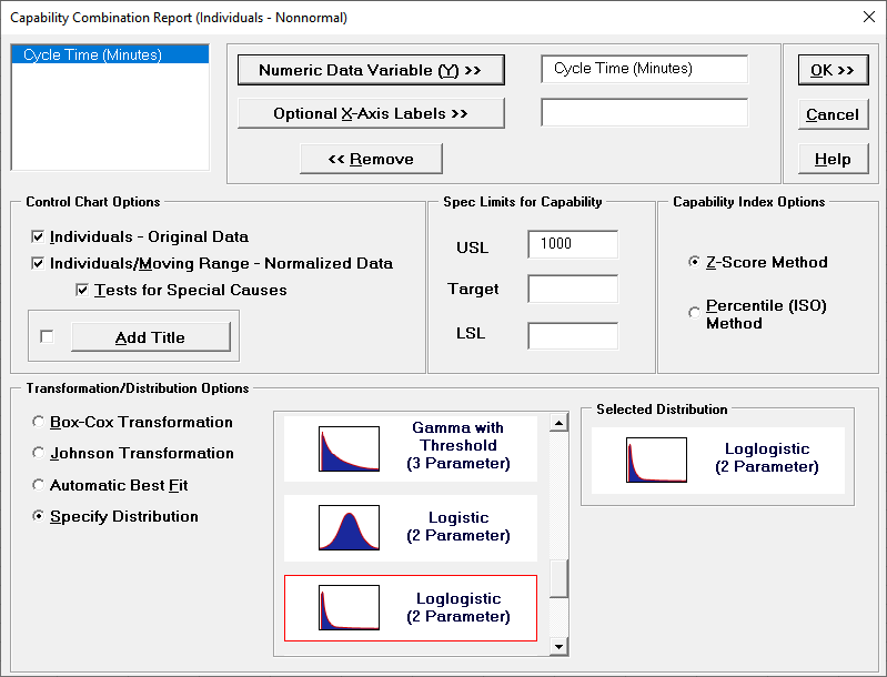
After reviewing this report, if you wish to perform a process capability analysis with a particular transformation or distribution, simply select Specify Distribution from the Transformation/Distribution Options in the Capability Combination Report (Individuals - Nonnormal) dialog as shown below (using 2 Parameter Loglogistic):

Click here to download a Free 30-Day Trial.