ARIMA Multiple Seasonal Decomposition (MSD) Control Chart

1. Open Monthly Airline Passengers – Modified for Control Charts.xlsx (Sheet 1 tab). This is based on the Series G data from Box and Jenkins, monthly total international airline passengers for January 1949 to December 1960. A Ln transformation is applied (avoiding the need for a Box-Cox transformation), a negative outlier is added at 50 (-.25) and a level shift applied (+.25), starting at 100. The Multiple Seasonal Decomposition (MSD) option is not necessary for this data, but by way of introduction, we will use this to compare to the previous analysis.
2. Click SigmaXL > Time Series Forecasting > ARIMA Control Chart > Multiple Seasonal Decomposition Control Chart. Ensure that the entire data table is selected. If not, Use Entire Data Table. Click Next.
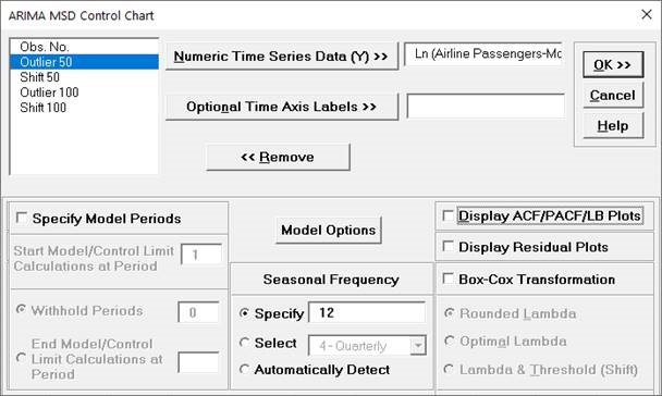
3. Select Ln(Airline Passengers-Modified), click Numeric Time Series Data (Y) >>. Uncheck Display ACF/PACF/LB Plots and Display Residual Plots. Check Seasonal Frequency with Specify = 12. Leave Specify Model Periods and Box-Cox Transformation unchecked.

   
   
   

4. Click Model Options.
   
   
   
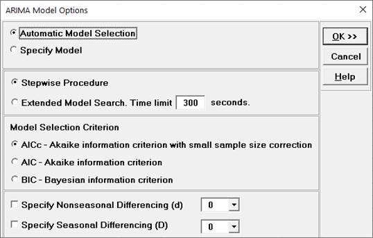
5. We will use the default Automatic Model Selection with AICc as the Model Selection Criterion. Click OK to return to the ARIMA Control Chart dialog. Click OK. The ARIMA (MSD) control charts are produced:
   
   
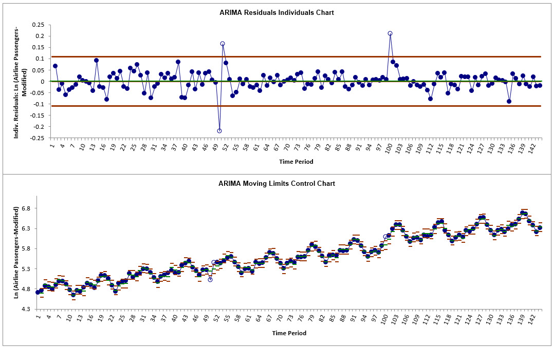
   We can clearly see the out-of-control data points at 50, 51 and 100 on the Residuals Individuals chart. This is similar to what we observed previously with regular ARIMA Control Charts.
   
   
6. Scroll down to view the ARIMA MSD Model header:
   
   
   
7. The ARIMA Model Summary is given as:
   
   
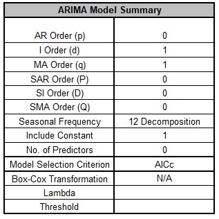   This is a summary of the model information for the deseasonalized data: ARIMA (0,1,1) with a constant. Seasonal Frequency = 12 using Decomposition and Model Selection Criterion = “AICc”. There are no seasonal terms in the model. The Box-Cox Transformation is “N/A”.
8. We will not review the Parameter Estimates, Model Statistics and Forecast Accuracy as they are close to the ARIMA MSD values given earlier, although note that slight differences are due to the introduction of an outlier and a shift, as well now we are using all of the data, i.e., there are no withhold periods. Earlier we used a Box-Cox Transformation with Lambda=0 and here we are using Ln of the data.
9. Open Half-Hourly Multiple Seasonal Electricity Demand - Taylor.xlsx (Sheet 1 tab). This is half-hourly electricity demand (MW) in England and Wales from Monday, June 5, 2000 to Sunday, August 27, 2000 (taylor, R forecast). This data has multiple seasonality with frequency = 48 (observations per day) and 336 (observations per week), with a total of 4032 observations. See the Run Chart, ACF/PACF Plots, Spectral Density Plot and Seasonal Trend Decomposition Plots for this data.
10.  We will first construct a classical Individuals Control Chart on the raw data. Click SigmaXL > Control Charts > Individuals. Ensure that the entire data table is selected. If not, check Use Entire Data Table. Click Next.
11. Select Demand, click Numeric Data Variable (Y) >>. Click OK. An Individuals Control Chart is produced:
    
    
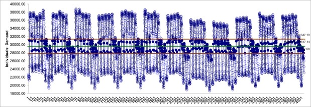    With the high frequency seasonality, this control chart is meaningless.
    
    
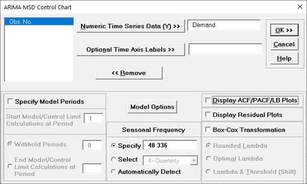
12. Click SigmaXL > Time Series Forecasting > ARIMA Control Chart > Multiple Seasonal Decomposition Control Chart. Ensure that the entire data table is selected. If not, check Use Entire Data Table. Click Next.
13. Select Demand, click Numeric Time Series Data (Y) >>. Uncheck Display ACF/PACF/LB Plots and Display Residual Plots. Check Seasonal Frequency with Specify = 48 336. Leave Specify Model Periods and Box-Cox Transformation unchecked.
    
    
    
14. Click Model Options.
    
    
    
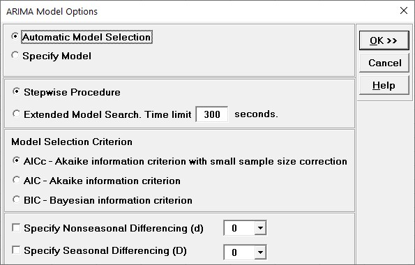
15. We will use the default Automatic Model Selection with AICc as the Model Selection Criterion. Click OK to return to the ARIMA MSD Control Chart dialog. Click OK. The ARIMA MSD control charts are produced:
    
    
    
16. Scroll down to view the ARIMA MSD Model header:
    
    
    
17. The ARIMA Model Summary is given as:
    
    
    
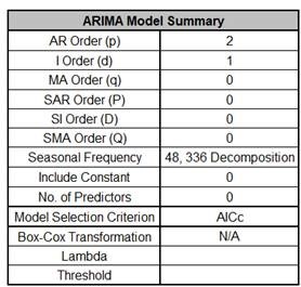
18. We will not review the Parameter Estimates, Model Statistics and Forecast Accuracy as they are close to the ARIMA MSD values given earlier, although note that now we are using all of the data, i.e., there are no withhold periods.

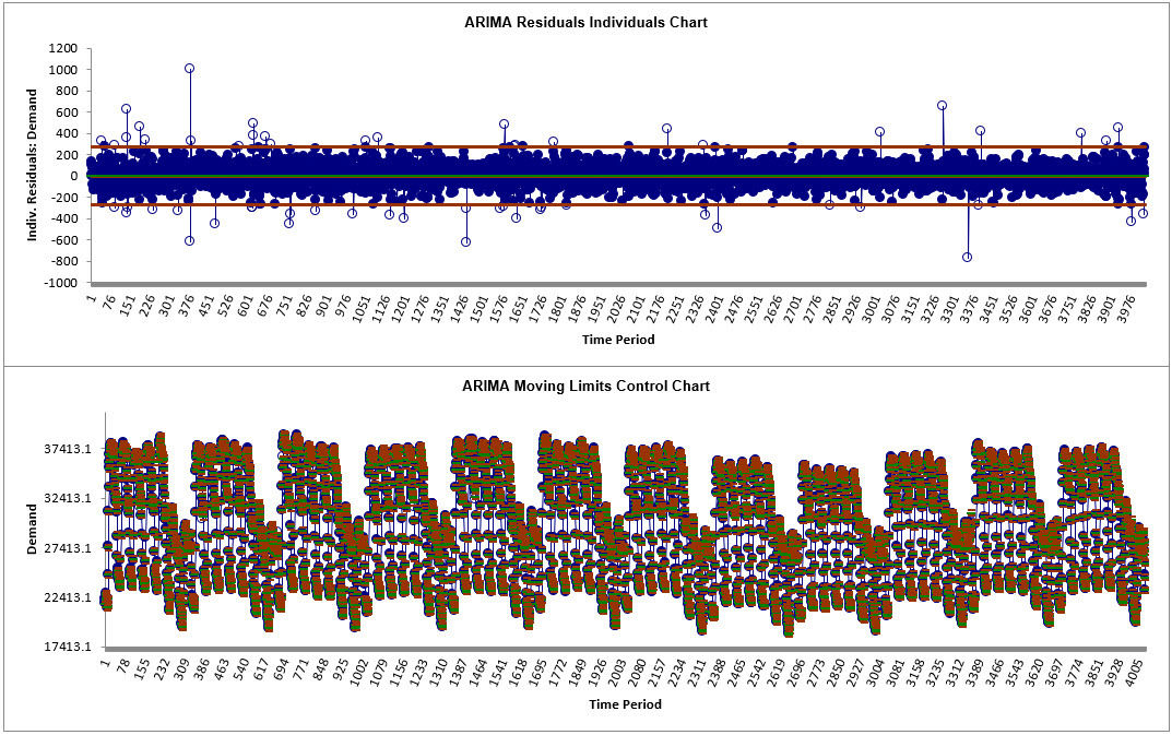
ARIMA does not have a theoretical frequency limit, but for computational efficiency and to minimize the potential loss of observations through differencing, we recommend using ARIMA – Multiple Seasonal Decomposition (MSD) for seasonal frequency greater than 52 (or with multiple frequencies). The seasonal component is first removed through decomposition, a nonseasonal ARIMA model fitted to the remainder (+trend), and then the seasonal component is added back in.

As the name implies, Multiple Seasonal Decomposition (MSD) also accommodates multiple seasonality, for example the half-hourly data with a seasonal frequency of 48 observations per day and 336 observations per week.

An Individuals control chart of the residuals is created for this forecast method. The Moving Limits chart uses the one step prediction as the center line, so the control limits will move with the center line. If a Box-Cox transformation is used then an inverse transformation is applied to calculate the control limits.

The popular “Add Data”, “Show Last 30” and “Scroll” features in SigmaXL Chart Tools are available for these control charts. For “Add Data”, the time series models are not refitted, but used to compute the residual values for the new data.